JCMT OT Basics

This tutorial is a basic introduction to the JCMT Observing Tool (OT). For further information, you may wish to refer to the following documentation:

• Installation instructions
• Full OT documentation

To complete this tutorial, you will need to download and unpack the example files.

• OT basics example files package

The package includes a completed version of the science program for exercise 1 which you can compare with your solution.

Downloading the OT

Before running the Observing Tool (OT), you must have Java installed. Please check your Java version as follows:

$ java -version
java version "1.8.0_121"
Java(TM) SE Runtime Environment (build 1.8.0_121-b13)
Java HotSpot(TM) 64-Bit Server VM (build 25.121-b13, mixed mode)

This should indicate that you are using Oracle’s version, “HotSpot”. The OT does not work properly with OpenJDK. If necessary, you can download the Java Runtime Environment (JRE) from Oracle’s website.

The OT is available as a single JAR file which you can download using the following link:

https://ftp.eao.hawaii.edu/ot/jcmtot.jar

If your system is not set up to automatically run JAR files, you can start it from a console as follows:

$ java -jar jcmtot.jar

If you are prompted to select a configuration, select “James Clerk Maxwell Telescope”.

1. Creating MSBs from the library

In this example we construct a science program based on MSBs from the library. For straightforward projects you can set up your program by simply taking library MSBs and customizing them to your needs.

1. Create a new science program. A science program contains the collection of all the observations which should be performed for a particular project.

   You can use either of the following methods:

   • Click the “Create New Program” button on the splash screen.
   • Select “File → New Program” from the menu of the (small) OT control window.

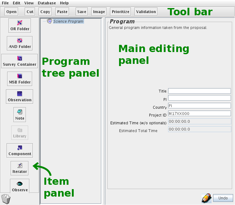
2. Take a moment to acquaint yourself with the OT interface. You will find:

   • At the top: a tool bar with common actions.
   • On the left: a panel of items which you can add to your program.
   • In the center: a panel showing a “tree” view of your program.
   • The main editing panel occupying the remainder of the window.

   

3. Fill in the program information for the top level “Science Program” item.

   Title

   A title for the program — usually the same as the proposal title.

   PI

   The project principal investigator. Enter your name here for this example.

   Country

   You can just enter “PI” here for the EAO PI science queue — this field is not important. (The label being “country” rather than “queue” is a historical oddity.)

   Project ID

   You can use a dummy ID such as M17XX000 for this example. When you store a science program to the OMP database, this ID is used to identify the project to which it belongs.

4. Open the SCUBA-2 library.

   • Select “File → Open SCUBA2 library” from the menu.

   Another OT window will open containing the library of sample SCUBA-2 observations, organized in a series of folders based on the type of observation. The observations are each contained in a structure called an MSB (minimum schedulable block). An MSB is the basic unit used to schedule observing time within a night at the JCMT. Everything within an MSB must be observable, and all its constraints met, for us to select it to be done at any point in the night.

   You can expand each item in the library to browse the MSBs and the structure within them.

5. Select the “point source daisy map” MSB (blue cube icon) and copy it to your new science program using the “Copy” and “Paste” buttons in the tool bar.

6. Expand each item in the tree panel of your new science program so that you can see the whole structure of the MSB.

7. Now you can go through the MSB and customize each item to your liking.

   Note

   This note (shown in blue and with the “show to the observer” box checked) will be shown to the telescope operator and observer when they perform the observation. You can include any information you wish them to be aware of regarding your program.

   Site quality

   Here you can choose “allocated” weather band and your observation will automatically be observed in any of the weather conditions approved by the time allocation committee for your project. It is also possible to further constrain the weather conditions by entering minimum and maximum opacity values (225 GHz, at zenith, labeled ‘τ’). Finally you can enter an opacity value to be used to compute noise estimates shown in the OT.

   DR recipe

   This component allows you to select the data reduction recipe which will be used to process your data. The selected recipe name will be written to a FITS header in raw data files. It is used by ORAC-DR for on-line reduction in the summit pipeline, in the reductions performed for the JCMT archive (at CADC) and as the default recipe when you run ORAC-DR manually. Since our example MSB is a type of scan observation, select the recipe you wish to use (e.g. “REDUCE_SCAN”) and press the “Set” button next to “Scan” to choose it.

   SCUBA-2

   This component selects SCUBA-2 as the instrument we wish to use. Since SCUBA-2 has no tuning configuration, this component is empty — it just has to be present to indicate that we are using SCUBA-2.

   Target information

   Enter the name of an astronomical target at the top of this panel. You can then either enter its coordinates manually, or try to look up the coordinates from the name using the “Resolve Name” button. SCUBA-2 observations just need the “SCIENCE” position, but in other types of observation, you may see additional entries in the table of positions, such as the “REFERENCE” position for heterodyne raster maps.

   Science observation

   This sets up an observation which is to be performed as part of the MSB. In this example, the MSB only has one observation. Note that this panel shows an estimate of the time taken to perform the observation. Each observation will always have a “Sequence” containing one or more actual observe actions.

   Scan

   This type of item (with an eye logo) triggers the telescope to do something. In this case, we are requesting a scan of an area of the sky. Note that the scan strategy “Point Source” is already selected — this corresponds to the daisy map pattern. For this strategy, the only configurable parameter is the integration time, which you can adjust to suit your target.

8. If you want to keep your work, you can save the science program to an XML file on your computer.

   • Select “File → Save As…” from the menu.

   If this were a real observing program, you would want to store the program in our database rather than (or as well as) saving it on your computer. In that case, the telescope systems make automatic updates to your program, such as indicating when MSBs have been observed, so it is important to always start by fetching the current version from our database rather than opening an old file you may have saved previously.

9. Finally it is always a good idea to validate your observing program.

   • Select the top level science program item in the program tree panel, because we want to check everything.
   • Click the “Validation” button in the tool bar.

   If successful, you should see a message saying:

   Science Program settings are valid.
   

2. Visualizing observations with the position editor

In this example we open an existing science program and visualize its observations using the position editor.

1. Open the 2_program.xml file.

2. Open the position editor window. There are three ways you can do this:

   • Click the “Image” button on the tool bar.
   • Select “View → Show the Position Editor” from the menu.
   • With a target information component selected, click the “Plot” button in the main editing panel.

3. Load the supplied image of Orion, 2_orion.fits, into the position editor. This can be done in one of the following ways:

   • Click the open button in the tool bar.
   • Select “File → Open” from the menu.

   Please note that the “JSky” software used for the position editor only supports certain types of FITS files — the example file has been prepared as described in the OT documentation.

4. With the default color levels, you will find that only the brightest emission in the center of the image can be seen.

   Adjust the color cut levels so that you can see more of the extended structure. You can open the cut level window in either of these ways:

   • Click the 4^th icon in the tool bar.
   • Select “View → Cut Levels” from the menu.

   Adjust the levels so that you can see more of the structure: the automatic 95% setting seems to work well for this image.

5. The position editor draws features related to the observations in pale colors. These can be easier to see with a plainer image color scheme.

   Open the image colors window:

   • Select “View → Colors” from the menu.

   Choose a simple color scheme such as “Red” or “Blue”.

6. Now we have the position editor set up, it’s time to start visualizing our observations.

   If you don’t already have a target information component selected, click the target information component for the first MSB in the program tree panel.

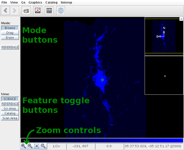
   Take note of controls which are now available in the panel at the left of the window:

   Mode buttons

   It is recommended that you use the tool only to visualize observations as you create them in the OT, keeping the “Browse” mode selected.

   Feature toggle buttons

   As you select different components in your science program, different features will be available for plotting. Here you can select which of these features are drawn. Ensure that the “SCIENCE” target position is enabled.

   

7. Take a look through the first MSB. The consists of three offset jiggle-chop observations taken along the northern filament.

   Select each item in turn and watch how the display in the position editor updates:

   Target information

   Since this is a chop (beam-switched) observation, the target information component does not include a reference position. The “Sci Area” feature shows the approximate field of view of the instrument.

   Offset

   This offset iterator defines a series of positions along the northern filament. You can plot them by selecting this component and then enabling the “Offset” feature in the position editor.

   Chop

   The chop iterator selects the beam-switching ‘throw’ (distance) and angle. When you select this component and enable plotting of the “Chop” feature, you will see a guide to how the chopping is performed. Unfortunately this is plotted at the science base position rather than our offset position. Note how the coordinate frame in our chop iterator has been set to “TRACKING”. This indicates that we wish to define the chop angle in the same coordinate system as that which the telescope is using to track our source — in this case J2000 coordinates since that is how the target has been defined. If you instead select “AZEL” (azimuth and elevation) coordinates, you will see the chop instead plotted as a circle, because the orientation in J2000 coordinates will vary depending on the time at which the source is observed.

8. Finally, take a look through the second MSB. This consists of a scan observation along the southern filament.

   Target information

   This observation is being performed with position-switching, so the target position nows includes the “REFERENCE” position. You can enable this feature in the position editor to see its location.

   Scan

   The scan item selects the size and angle of the area to be scanned. If you select this component you will be able to enable plotting of the “Scan Area” feature. As for the chop iterator, this is unfortunately plotted at the science base position.

   Offset

   This defines a position on the southern filament which will be used as the center of the scan area. Plotting the “Offset” feature here also includes a box showing the offset scan area.