This is an introductory tutorial to JCMT data reduction, including the following topics:
The examples in this tutorial will assume that you have the Starlink software installed and set up by sourcing the relevant profile file. For example if you have unpacked the Starlink 2023A release as star-2023A in your home directory, you can do:
export STARLINK_DIR=~/star-2023A
source $STARLINK_DIR/etc/profile
If you are using csh or tcsh, you will need to source the cshrc and login files instead:
setenv STARLINK_DIR ~/star-2023A
source $STARLINK_DIR/etc/cshrc
source $STARLINK_DIR/etc/login
If you have not already done so, unpack the tutorial tar package and change into its directory:
tar -xzf tutorial_prp.tar.gz
cd tutorial_prp
Next we configure ORAC-DR to process SCUBA-2 850μm data using the oracdr_scuba2_850 alias.
oracdr_scuba2_850
This in turn sets up the oracdr (and wesley) aliases. It also defines a number of environment variables including two important directory paths:
The default values for these paths will be set appropriately for the computer systems at JCMT, so we will need to adjust them. It is also possible to specify --cwd to set ORAC_DATA_OUT to the current directory.
export ORAC_DATA_IN=`pwd`/raw-data
Our first observation is a SCUBA-2 flux calibrator (CRL 2688). However when this observation was taken, a fault prevented opacity data from the JCMT WVM from being attached to the raw data. Attempting to reduce this observation directly results in an error:
#12 Err: !! Unable to determine opacity data for this observation. WVM data missing or
#12 Err: !     entirely unusable. 0 % of WVM data are present (0 % before despiking).
In order to handle this observation, we will use Wesley to insert the WVM data. Wesley is a pre-processing pipeline with recipes to handle some common problems with raw data. Hopefully you will never have to use it on your own data, but more details are available in SUN/271.
First make a new directory in which to do the processing, move into it, and set ORAC_DATA_OUT to this directory.
mkdir reduced-scuba2-cal
cd reduced-scuba2-cal

export ORAC_DATA_OUT=`pwd`
Then we can run Wesley. We must specify the pre-processing recipe we wish to run, in this case INSERT_JCMT_WVM_DATA. We also specify a number of command line options:
wesley --log sf --nodisplay --files ../raw-data/in-scuba2-cal.lis \
    --recpars JCMT_WVM_DIR=../raw-data/wvm \
    INSERT_JCMT_WVM_DATA
We have specified the files to be processed via the --files command line option and a listing in-scuba2-cal.lis. This can contain full path names, or names relative to ORAC_DATA_IN. In this case, it contains:
raw-scuba2-cal/s8a20230108_00012_0001.sdf
raw-scuba2-cal/s8a20230108_00012_0002.sdf
raw-scuba2-cal/s8a20230108_00012_0003.sdf
raw-scuba2-cal/s8a20230108_00012_0004.sdf
raw-scuba2-cal/s8a20230108_00012_0005.sdf
raw-scuba2-cal/s8a20230108_00012_0006.sdf
raw-scuba2-cal/s8a20230108_00012_0007.sdf
This listing was created by doing ls raw-scuba2-cal/* > in-scuba2-cal.lis in the raw-data directory.
The pipeline will write several lines of log output. You will see that it has copied each raw file to a new file with a _wvm suffix and then inserted the JCMT WVM data into the new file.
Using recipe INSERT_JCMT_WVM_DATA specified on command-line
Determined TAI offset from header: 37.0 seconds
Reading JCMT WVM data from file ../raw-data/wvm/20230108.wvm
Inserting WVM data into file s8a20230108_00012_0001_wvm
Inserting WVM data into file s8a20230108_00012_0002_wvm
Inserting WVM data into file s8a20230108_00012_0003_wvm
Inserting WVM data into file s8a20230108_00012_0004_wvm
Inserting WVM data into file s8a20230108_00012_0005_wvm
Inserting WVM data into file s8a20230108_00012_0006_wvm
Inserting WVM data into file s8a20230108_00012_0007_wvm
Writing preprocessed file list to preproc_2877.lis
Recipe took 10.529 seconds to evaluate and execute.
This output also indicates that a new file listing was generated. Note that the name of this file will change to include the current process ID — you will need to identify the file generated by your run of Wesley. (The file name can also be controlled via the WESLEY_FILE_LIST recipe parameter.)
We can pass the file listing written by Wesley to ORAC-DR to continue with the data reduction:
oracdr --log sf --nodisplay --files preproc_2877.lis
This will produce a number of files, including:
You can examine the reduced products using GAIA. Note the & at the end of the command to launch GAIA in the background:
gaia s20230108_00012_850_reduced.sdf &
An alternative would be simply to open the preview PNG images.
We now have an adequate image of our calibrator, but it would be nice to extract just the section around the target source. We can do this using the PICARD recipe CROP_SCUBA2_IMAGES. The most common way to run PICARD is to give one or more files (with the .sdf file extension) directly on the command line, for example:
picard --log sf CROP_SCUBA2_IMAGES s20230108_00012_850_reduced.sdf
We can send the cropped image into our existing GAIA window with the gaiadisp command:
gaiadisp s20230108_00012_850_reduced_crop.sdf
The cropping process can be controlled with recipe parameters. For example, to extract a circular area rather than the default rectangular area:
picard --log sf --recpars CROP_METHOD=circle,MAP_RADIUS=120 CROP_SCUBA2_IMAGES \
    s20230108_00012_850_reduced.sdf
More details about PICARD can be found in SUN/265. A few PICARD recipes you could try running on our calibrator map are:
For each instrument, ORAC-DR includes a selection of different recipes designed to be used with different types of target sources. For SCUBA-2, details of these recipes can be seen in SUN/264. You can select a data reduction recipe in the DRRecipe component of the JCMT Observing Tool when initially setting up your observation. When you do this, the name of the chosen recipe will be written into the RECIPE FITS header of raw data files, for example:
RECIPE = 'REDUCE_SCAN' / ORAC-DR recipe
In this section of the tutorial, we will be looking at an observation of NGC 1333 taken as part of the JCMT Transient Survey. This was a large pong map, but it has bright and extended structure so we only need to reduce a small sample of the data to begin to see the differences between the various recipes.
First return to the top level directory of the tutorial:
cd ..
Or if you are starting at this section, initalize Starlink and ORAC-DR then define ORAC_DATA_IN:
export STARLINK_DIR=~/star-2023A
source $STARLINK_DIR/etc/profile
oracdr_scuba2_850
export ORAC_DATA_IN=`pwd`/raw-data
First we will try the default recipe, REDUCE_SCAN. This uses a makemap configuration file dimmconfig_jsa_generic.lis designed to work reliably on a variety of different sources. (More on makemap configuration later.)
To allow us to compare different reductions, we can create a new directory, set ORAC_DATA_OUT to this directory, and then launch ORAC-DR. This will cause ORAC-DR to change into the specified directory and then perform the reduction there. (Specifying REDUCE_SCAN is not strictly necessary here as it is the recipe given in the FITS headers.)
mkdir reduced-scuba2-default
export ORAC_DATA_OUT=`pwd`/reduced-scuba2-default
oracdr --log sf --nodisplay --files raw-data/in-scuba2-ngc1333.lis REDUCE_SCAN
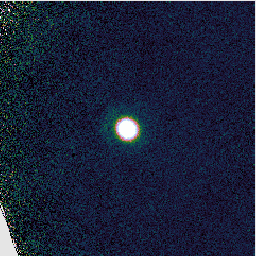
You can open the reduced data files in GAIA, as before, to inspect the results. You should find that it has produced a fairly typical SCUBA-2 reduction. (The unusual square shape is because we only included a small section of the pong map pattern.)
Another recipe is REDUCE_SCAN_ISOLATED_SOURCE. This is designed for maps with a small isolated source at the target position and blank sky elsewhere. Again we can run the reduction in a separate directory:
mkdir reduced-scuba2-isolated
export ORAC_DATA_OUT=`pwd`/reduced-scuba2-isolated
oracdr --log sf --nodisplay --files raw-data/in-scuba2-ngc1333.lis REDUCE_SCAN_ISOLATED_SOURCE
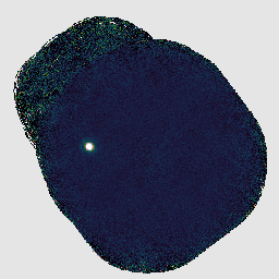
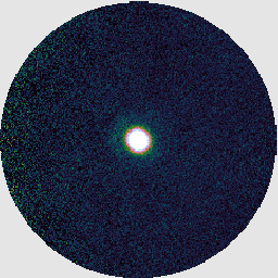
If you look at the resulting map with GAIA, you should find negative stripes or bowling around the bright sources. This has happened because this recipe uses a makemap configuration file dimmconfig_bright_compact.lis which restricts the AST model to the central 60″. (This is the area of the circle cut out of the image on the right below.) The makemap program will therefore not be expecting emission outside of this region. This recipe is clearly a poor match to our observation!
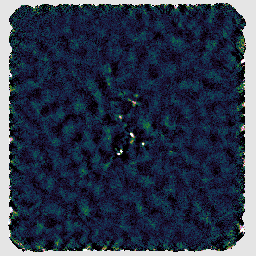
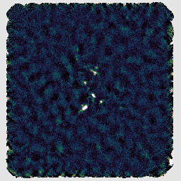
A recipe which can be used to attempt to recover more extended structure is REDUCE_SCAN_EXTENDED_SOURCES. This includes various changes, including increasing the filtering scale from 200″ to 480″.
mkdir reduced-scuba2-extended
export ORAC_DATA_OUT=`pwd`/reduced-scuba2-extended
oracdr --log sf --nodisplay --files raw-data/in-scuba2-ngc1333.lis REDUCE_SCAN_EXTENDED_SOURCES
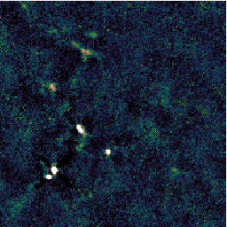
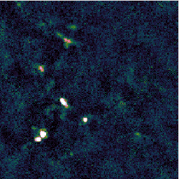
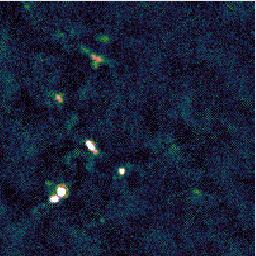
You may find that this recipe has preserved more structure around some of the bright sources, at the expense of a less flat background, as in the image on the left below. Recovering extended structure is difficult from our sample data which only includes one of SCUBA-2's sub-arrays, since we are not using the full field of view of the instrument. Performing this reduction on the data from all sub-arrays would give the central image below. Including the whole observation gives the image on the right.
The final recipe we will try is REDUCE_SCAN_FAINT_POINT_SOURCES. This is intended for observations such as cosmology fields where faint point sources are expected anywhere in the map.
mkdir reduced-scuba2-faint
export ORAC_DATA_OUT=`pwd`/reduced-scuba2-faint
oracdr --log sf --nodisplay --files raw-data/in-scuba2-ngc1333.lis REDUCE_SCAN_FAINT_POINT_SOURCES
With this recipe, the matched filter is automatically applied to the group product. This includes smoothing which will emphasize point sources.
As we have seen, part of the difference between the various data reduction recipes is the usage of a different makemap configuration file. ORAC-DR passes these files to the makemap program which is responsible for the initial processing of the raw SCUBA-2 data to create a 2D map. There is a very large number of parameters which can be adjusted in this way — a full list of configuration parameters is given in Appendix E of SUN/258.
In the configs directory you should find a file pca.lis intended to enable the PCA model in makemap. It contains the following configuration:
^$STARLINK_DIR/share/smurf/dimmconfig_jsa_generic.lis
^$STARLINK_DIR/share/smurf/dimmconfig_pca.lis

# Main parameter controlling the PCA process. If negative, the
# absolute value gives the number of components to remove.
pca.pcathresh = -8

# Reduce number of iterations to complete this example faster.
numiter = -15
In configuration files like this you will find:
You may find you do not need as many PCA components as specified by dimmconfig_pca.lis. This configuration reduces the number of components to 8. It also restricts the number of iterations to be performed by makemap to 15 for the purposes of this tutorial. The reduction would likely require more iterations than this to converge.
We can give our configuration file to ORAC-DR using the recipe parameter MAKEMAP_CONFIG. (We give the full path name here because ORAC-DR will look for the file after moving into ORAC_DATA_OUT.)
mkdir reduced-scuba2-pca
export ORAC_DATA_OUT=`pwd`/reduced-scuba2-pca
oracdr --log sf --nodisplay --files raw-data/in-scuba2-ngc1333.lis \
    --recpars MAKEMAP_CONFIG=`pwd`/configs/pca.lis \
    REDUCE_SCAN
Warning: this example should only be run on a system with at least 6, or preferably 8, CPU cores. (Performance of the PCA model currently seems very poor with fewer threads than this, becoming practically unusable with 4 or fewer, although it is possible to specify a higher number of threads, e.g. with export SMURF_THREADS=8.)
If you examine the reduced image in GAIA, you should hopefully find that including PCA has cleaned the background somewhat compared to the default reduction with REDUCE_SCAN, as in the image below.
There are a couple of blog posts describing the usage of PCA in SMURF:
Finally to end this section on SCUBA-2 data reduction we should mention a couple more common recipe parameters. If you wish, you may experiment with setting these values via the --recpars command line option:
Detailed information about the recipes available for SCUBA-2 and their parameters is given in SUN/264.
In this section we will look at two heterodyne observations. These are both jiggle maps made using the receiver HARP and the ACSIS backend, targeting the CO 3–2 spectral line.
ORAC-DR works very similarly for ACSIS data as for SCUBA-2. We start by initializing it using the oracdr_acsis alias. After re-initializing ORAC-DR, we will also need again to ensure that ORAC_DATA_IN is set correctly.
oracdr_acsis
export ORAC_DATA_IN=`pwd`/raw-data
Our first observation is of an HII region. As in the previous examples, we can have ORAC-DR run in a sub-directory to keep the output files separate. We can just give ORAC-DR the file list via --files and allow it to select a recipe based on the RECIPE FITS header:
mkdir reduced-harp-hii
export ORAC_DATA_OUT=`pwd`/reduced-harp-hii
oracdr --log sf --nodisplay --files raw-data/in-harp-hii.lis
As ORAC-DR starts processing, you will see it write out the name of the selected recipe:
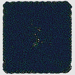
REDUCING: a20181202_00013_01_0001
Using recipe REDUCE_SCIENCE_NARROWLINE provided by the frame
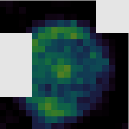
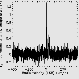
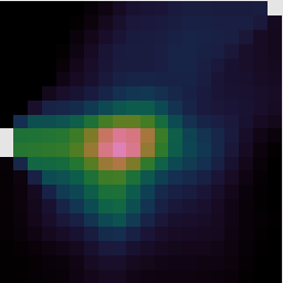
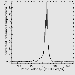
It will produce several output files. The main ‘reduced’ products are data cubes and representative images and spectra are extracted in order to give a preview of the data.
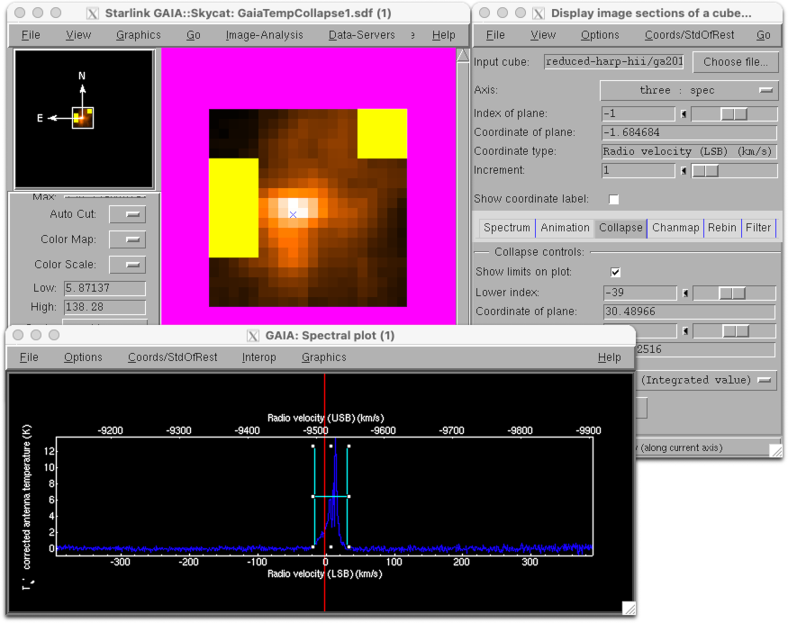
If you open the reduced data cube in GAIA you will be able to zoom in using the big Z button. You can click any point in the cube to see the spectrum at that position, and drag the red bar in the spectrum to change the image to display the corresponding spectral channel.
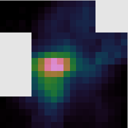
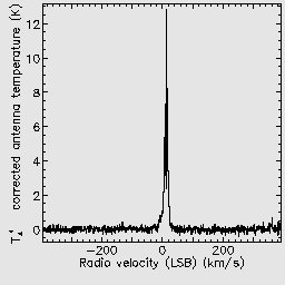
You can also interact with data cubes in GAIA using the cube toolbox window which appears. For example from the Collapse tab you can select a spectral range over which to collapse the data. Ticking the Show limits on plot box allows you to see the part of the spectrum which will be collapsed in the pop-up Spectral plot window.
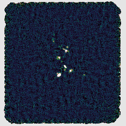
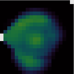
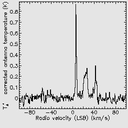
You may also try reducing a second observation, which is a jiggle map of U Ant. You should again see that ORAC-DR is using the recipe REDUCE_SCIENCE_NARROWLINE.
mkdir reduced-harp-uant
export ORAC_DATA_OUT=`pwd`/reduced-harp-uant
oracdr --log sf --nodisplay --files raw-data/in-harp-uant.lis
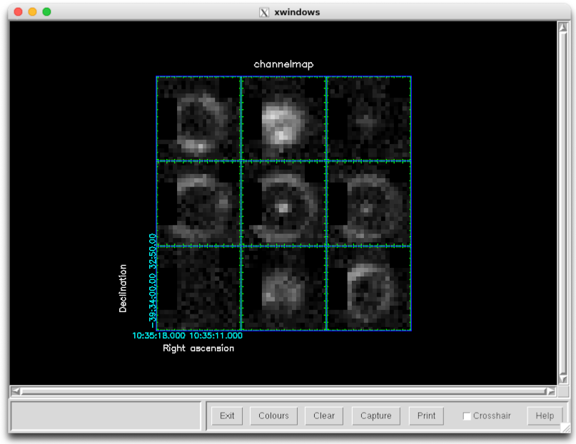
You can examine the resulting data products in GAIA as before. However it is also possible to use other Starlink software packages for futher analysis. For example the chanmap command from KAPPA can be used to create a series of channel maps. Here we initialize KAPPA with the kappa command, create 9 channel maps from 0 to 50 km/s, and then display them:
kappa
chanmap in=ga20190101_47_1_reduced001 out=channelmap \
    axis=3 nchan=9 shape='!' low=0 high=50
display channelmap dev=xwin mode=fa
The behavior of many recipes can be controlled via recipe parameters. We have already seen examples of giving one or two parameters directly via the --recpars command line options. However when you want to specify several parameters, or re-use them for different reductions, it is more convenient to store them in a recipe parameter file.
In the recpars directory you should find a file acsis-smooth.ini which contains the text below. This file is in .ini format, where the section names, which are enclosed in square brackets ([…]), correspond to ORAC-DR recipe names. Since our observations use the recipe REDUCE_SCIENCE_NARROWLINE, our parameters are listed in a section identified with [REDUCE_SCIENCE_NARROWLINE]. (Sections can also specify a target object or other details of the observation — see section 6.2 of SC/20 for more details.) In this way it is possible to use one file to store different parameters for multiple different recipes.
[REDUCE_SCIENCE_NARROWLINE]
SPREAD_METHOD = gauss
SPREAD_WIDTH = 24
SPREAD_FWHM_OR_ZERO = 12
FINAL_LOWER_VELOCITY = -100
FINAL_UPPER_VELOCITY = 100
These parameters indicate that the cube should be gridded using a very large Gaussian spread function, and that the final output should be restricted to a velocity range of -100 to 100 km/s.
If you repeat the previous reductions, but with this recipe parameter file, you should be able to see the smoothing effect which has been caused by the Gaussian regridding.
mkdir reduced-harp-hii-sm
export ORAC_DATA_OUT=`pwd`/reduced-harp-hii-sm
oracdr --log sf --nodisplay --files raw-data/in-harp-hii.lis --recpars recpars/acsis-smooth.ini

mkdir reduced-harp-uant-sm
export ORAC_DATA_OUT=`pwd`/reduced-harp-uant-sm
oracdr --log sf --nodisplay --files raw-data/in-harp-uant.lis --recpars recpars/acsis-smooth.ini
Here are a few more ACSIS recipe parameters which you could experiment with:
You can find more about the recipes available for ACSIS and their parameters in SUN/260. There is also a categorized list of recipe parameters in Appendix G of SC/20.
Additional calibration override parameters can be given via the --calib command line option. One such parameter is bad_receptors which can be used to control how the pipeline should exclude bad receptors. This can be a colon-separated list of receptor names to excluded, which can be useful if you wish to remove some poorly performing receptors, or reduce only one polarization of Nāmakanui data.
For example the remaining corner receptors can be excluded by adding this option to an oracdr command:
--calib bad_receptors=H03:H12:H15
Finally, for completeness, other commonly-used ACSIS recipes are listed below. These typically differ in the expected spectral features and therefore how the pipeline should identify suitable regions to which to fit a baseline.
This is an additional section of the tutorial in case you have more time available.
Starlink includes a number of dimmconfig files containing configuration parameters for makemap in the share/smurf directory. You can see them all as follows:
ls $STARLINK_DIR/share/smurf/dimmconfig*
This directory includes some configurations intended for specific purposes:
dimmconfig_blank_field.lis
dimmconfig_bright_compact.lis
dimmconfig_bright_extended.lis
dimmconfig_jsa_generic.lis
dimmconfig_moon.lis
dimmconfig_pointing.lis
dimmconfig_veryshort_planet.lis
And some ‘add-on’ files which you can include in your configuration:
dimmconfig_fix_blobs.lis
dimmconfig_fix_convergence.lis
dimmconfig_pca.lis
First re-initialize ORAC-DR for SCUBA-2:
oracdr_scuba2_850
export ORAC_DATA_IN=`pwd`/raw-data
Now we can try reducing data using the example file configs/parameters.lis which includes values based on dimmconfig_jsa_generic.lis and dimmconfig_fix_blobs.lis. The comments in this file show some commonly-used values.
# Maximum number of iterations and convergence criterion.
numiter = -25
maptol = 0.01

# Enable to store the map at the end of each iteration in the output file.
# [Warning: will greatly increase the output file size.]
# itermap = 1

# Reject bolometers noisier than this (standard deviations).
# [Increase to cope with bright sources, default: 4]
noisecliphigh = 10.0

# S/N threshold to detect DC steps in bolometer time series.
# [Again increase for bright sources, default: 25]
dcthresh = 100

# Evaluate COM (common mode) model on each sub-array individually.
# [Will have no effect on our test data which only includes one sub-array.]
com.perarray = 1

# Filter out large scale structure (size in arcseconds).  This is applied
# to the bolometer time series as an equivalent time (based on the scan speed).
# [E.g. 100 (smallest) - 480 (extended structure)]
flt.filt_edge_largescale = 200

# Use an automatic AST (astronomical signal) model mask generated at
# ast.zero_snr (sigma) traced down to ast.zero_snrlo (sigma).
# [Typically snr 3 - 5 to snrlo 1.5 - 3 sigma]
ast.zero_snr = 5
ast.zero_snrlo = 3

# Apply similar masking to the FLT (filter) model.
flt.zero_snr = 5
flt.zero_snrlo = 3

# Skip usage of the AST model for this many iterations to allow
# COM and FLT masks to become established (if in use).
ast.skip = 5

# Alternatively mask a small circle at the target position for compact objects.
# [E.g. 0.016666 deg = 60" - 0.033333 = 120".]
# ast.zero_circle = (0.016666)
# flt.zero_circle = (0.016666)

# These parameters from dimmconfig_fix_blobs.lis are intended to reduce
# ringing from the FLT model.
flt.filt_order = 4
flt.ring_box1 = 0.5
A full list of configuration parameters is given in Appendix E of SUN/258. There is also a categorized list in Appendix J of SC/21.
We can use what we saw in the last section to conveniently load this configuration via a recipe parameter file. The file recpars/scuba2-parameters.ini simply specifies our configuration file for the REDUCE_SCAN recipe:
[REDUCE_SCAN]
MAKEMAP_CONFIG=../configs/parameters.lis
Then as before we run the pipeline writing into a new directory:
mkdir reduced-scuba2-param
export ORAC_DATA_OUT=`pwd`/reduced-scuba2-param
oracdr --log sf --nodisp \
    --recpars recpars/scuba2-parameters.ini \
    --files raw-data/in-scuba2-ngc1333.lis
This gives a perhaps slightly improved result as compared to the default reduction:
When experimenting with configuration parameters, you can use separate directories to retain and compare the results, or simply use the same directory and then have GAIA load the new map with the File → Reopen menu option.
There are several ways we can monitor the performance of the data reduction. The first is to simply give the --verbose command line option to ORAC-DR. This will cause it to include in its log the messages output by the underlying makemap application. These include, for example, statistics reported at each iteration of the map-making process.
smf_iteratemap: Iteration 19 / 25 ---------------
smf_iteratemap: Calculate time-stream model components
smf_iteratemap: Rebin residual to estimate MAP
smf_iteratemap: Calculate ast
--- Quality flagging statistics --------------------------------------------
 BADDA:   11342686 (31.33%),         401 bolos  ,change          0 (+0.00%)
BADBOL:   11597260 (32.03%),         410 bolos  ,change          0 (+0.00%)
 SPIKE:          5 ( 0.00%),                    ,change          0 (+0.00%)
DCJUMP:        511 ( 0.00%),                    ,change          0 (+0.00%)
  STAT:      38400 ( 0.11%),          30 tslices,change          0 (+0.00%)
   COM:     558962 ( 1.54%),                    ,change          0 (+0.00%)
 NOISE:      28286 ( 0.08%),           1 bolos  ,change          0 (+0.00%)
  RING:    3529862 ( 9.75%),                    ,change          0 (+0.00%)
Total samples available for map:   20724010, 57.24% of max (732.66 bolos)
     Change from last report:          0, +0.00% of previous
smf_iteratemap: *** CHISQUARED = 0.939922406253459
smf_iteratemap: *** change: -7.42441147449924e-08
smf_iteratemap: *** NORMALIZED MAP CHANGE: 0.00662308 (mean) 0.0443517 (max)
We can also examine the quality flags attached to the output map. The KAPPA command showqual will list these flags:
kappa
showqual gs20151222_18_850_reduced
AST (bit 1) - "Set iff AST model is zeroed at the output pixel"
FLT (bit 2) - "Set iff FLT model is not blanked at the output pixel"
In this case we have quality flags related to the AST and FLT models. Examining these will allow us to see the effect of the corresponding parameters such as ast.zero_snr and ast.zero_snrlo.
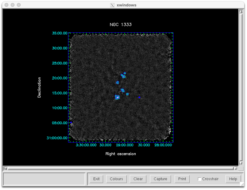
We can display the quality array in GAIA by choosing it in the Select NDF… window. Alternatively we can use KAPPA to mask the map based on the quality flags and then use contour … mode=good to outline the relevant areas:
qualtobad gs20151222_18_850_reduced gs20151222_18_850_reduced_ast ast
qualtobad gs20151222_18_850_reduced gs20151222_18_850_reduced_flt flt

display gs20151222_18_850_reduced mode=fa dev=xwin

contour gs20151222_18_850_reduced_flt mode=good dev=xwin \
    noclear style="'colour(curves)=blue,width(curves)=10'"
contour gs20151222_18_850_reduced_ast mode=good dev=xwin \
    noclear style="'colour(curves)=green,width(curves)=2'"
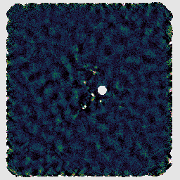
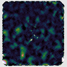
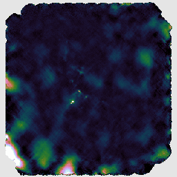
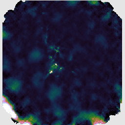
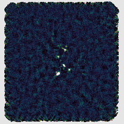
Finally if we enable the itermap configuration parameter then makemap will store a map at the end of each iteration. If a map has problematic features then this will allow you to see how they develop during processing. We can combine the iteration maps into a cube using the SMURF command stackframes and then open the cube in GAIA in order to scroll through it.
smurf
stackframes gs20151222_18_850_reduced.MORE.SMURF.ITERMAPS out=itermaps nosort
Here is the center of the map from the first three iterations: