Finding and correcting DC jumps
Sudden changes in the DC level are seen to occur within bolometer time
streams. The following algorithm attempts to identify and correct these
steps. Each bolometer time stream is processed independently using the
following two part process
Part 1 - Detecting Candidate Steps:
In this part we search the bolometer time stream for contiguous blocks
of samples that have unusually large gradients compared to the
neighbouring samples. Each such block of samples is considered to be a
candidate DC jump. The starting and ending time of each such block is
noted. Once all candidate jumps have been found for a bolometer, the
algorithm proceeds to part 2. Candidate jumps are found as follows:
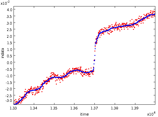
- Smooth the bolometer time stream using a median filter of width
DCSMOOTH (defaults to 50) samples. This reduces the effects of the
noise in the data. Using a median filter rather than a
mean filter helps to preserve the sharp edges at each DC jump, and is
robust against spikes, etc. The following figure shows a typical
step, with the original bolometer data values in red and the
median-smoothed data values in blue.
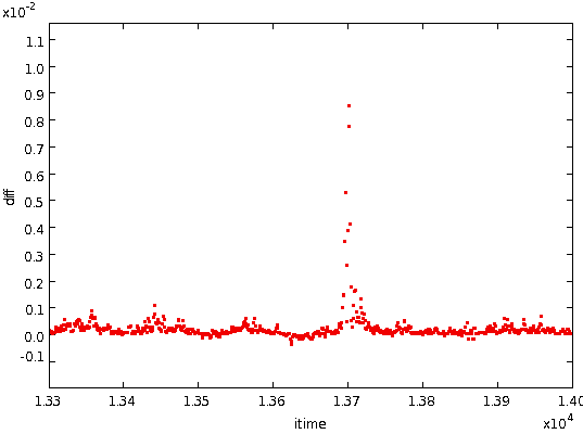
- At each sample, find the difference between the two adjacent
values in the median filtered bolometer data. This is proportional to
the gradient of the median filtered bolometer data. These gradients
include both the gradient of the underlying noise free median-filtered
data stream ,and the extra gradient caused by noise, spikes, DC jumps,
etc. The following figure shows these differences for the above step.
The high gradients at the step are clearly visible.
- We now need to split these differences up into differences caused
by variation of the underlying noise-free data, and differences
caused by noise, steps, spikes, etc.To do this we smooth the above
differences, and use the smoothed differences as the gradient of the
underlying noise free data. In order to get an accurate result, we need
to do this smoothing with a mean filter rather than a median filter.
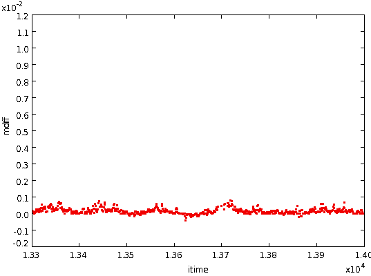
But a mean filter is badly affected by aberrant values, so we first
take a copy of the differences found above, and remove extremely
large differences by flagging them as bad. Specifically, differences
more than three times the RMS difference (taken over the whole time
stream) are set bad. The RMS is then
re-calculated and a further two such rejection iterations are
performed. This gets rid of high gradient values caused by
spikes, jumps, point sources, etc, leaving the following:
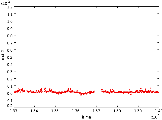
- The differences close to a step are often not typical of those in
the wider neighbourhood, so each block of contiguous values removed
above is doubled in width, leaving the following:
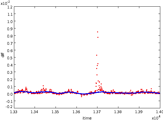
- Smooth the remaining differences using a mean filter
of width DCSMOOTH. The smoothing process fills in small holes in
the array (up to 0.8*DCSMOOTH), but will not fill in larger holes. Such
larger holes are filled in by linear interpolation. The resulting
smoothed differences - shown in blue below overlayed on the original
differences in red - estimate the
local gradient of the underlying noise-free median-filtered data
stream.
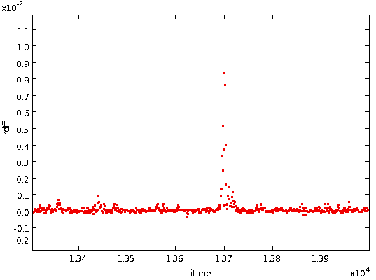
- Subtract the smoothed differences from the total differences
found in
step 2 above. This gives the residual differences caused by noise,
spikes, DC jumps, etc., shown below:
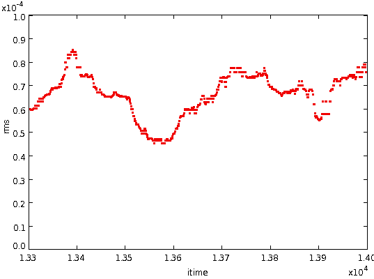
- To decide if a residual difference value is "unusually high" we
need an estimate of the local RMS of these residual differences at each
point in the data
stream. To get this we smooth the squared residual gradients using a
median filter
of width DCSMOOTH2 (fixed at 200), and then take the square root of the
resulting values.
- Divide the residual differences by the local RMS of the residual
differences to get a "signal-to-noise" ratio for each residual
difference value:
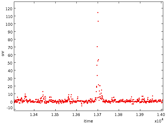
- Find all blocks of contiguous absolute SNR values greater than
DCTHRESH (defaults to 25). Such blocks
are allowed to contain small numbers of values that do not
meet this criterion. The maximum length for such a section of low
SNR is DCFILL (fixed at 40) samples. For the example step shown above,
the
block starts at 13696 and ends at 13703. Blocks are ignored if they
fail any of the following tests:
- The width of the block must be less than DCMAXWIDTH (fixed at
60)
- The total of all the SNR values in the block must be at least
DCTHRESH. This test avoids spikes being treated as two very close
steps, since such steps will have SNR values of opposite signs
and will thus cancel out.
- The total of all SNR values in the block must exceed half the
value of the largest single SNR value in the block.
- (this tends to rejects spikes since they will have large
positive and negative SNR values within the block, which will cancel
out).
Part 2 - Measuring and Correcting Steps
In this part, each of the candidate steps found above is processed
to determine the height of the step. This is done by doing a
least squares linear fit to the median-smoothed bolometer data just
before the step, and another fit to the data just after the step. These
two fits are used to predict the value at the centre of the step, and
the difference between these two predicted values is used as the step
height. Various other tests are performed to identify and reject
spurious step detections, and finally the original bolometer data
stream is corrected to take out the step. For a given bolometer, each
candidate step is processed as follows:
- Correct the step start and end to include adjacent SNR values that are below DCTHRESH but are still significantly high. Specifically, the step start is moved to the end of the last block of DCNLOW (fixed at 5) SNR values that are all less than DCSIGLOW (fixed at 8.0), and which occurs before the original step start. Likewise, the step
end is moved to the start of the earliest block of DCNLOW SNR values
that are all less than DCSIGLOW, and which occurs after the original
step end.For the example step shown above, the start moves from 13696 to 13693, and the end moves from 13703 to 13711.
- Perform a linear fit to the median-smoothed bolometer data before
the step. The fit is over a box containing DCFITBOX (defaults to30) samples. A gap of DCFITBOX samples is left between the end of the box and the start of the step.
- Perform a linear fit to the median-smoothed bolometer data after
the
step. The fit is over a box containing DCFITBOX samples, and a gap of
DCFITBOX samples is left between the end of the step and the start of
the box.
- These two fits are evaluated at the centre of the step. The
difference between these values gives an estimate of the step height.
However, moving the fitting box slightly can often result in big
changes in the line gradient, and thus big changes to the estimate of the jump height. Steps where this is the case are ignored (i.e. left unfixed).
To check this, more linear fits are performed at increasing distances
from the step, and the consistency of the estimated jump heights from
these extra fits is checked. Specifically, the fitting box used in step
2) above is moved one sample earlier, a new fit is performed, and
the new fit is used to estimate the value at the centre of the
step. The fitting box is then moved again by one sample and a
third fit performed giving a third estimate of the central data value.
This process is repeated until we have performed 2*DCFITBOX fits (an
efficient algorithm is used to perform these multiple fits). The
variance of all these estimates of the central value is found. The same
thing is then done to the fit performed in step 3) above, to give us
the variance of the central data value determined from the data
following the step. The uncertainty in the jump height is then taken to
be the square root of the mean of the two variances values, and the
jump is ignored if the jump height - determined from steps 2) and 3) - is less than DCTHRESH2 (fixed at 1.5) times the uncertainty in the jump height.
- The jump is also ignored if it is less than DCTHRESH3 (fixed at 4.0) times the noise in the original bolometer data. The bolometer noise value used is the RMS of the differences between adjacent bolometer values, excluding aberrant points, and corrected by a factor of 1/sqrt(2).
- If the step is not rejected, all the original bolometer
values following the centre of the step are adjusted upwards or
downwards by the step height.
Once all steps have been corrected, a constant value is added back on
to all bolometer samples so that the original mean value in the
bolometer is retained.