The JCMT Observing Tool

Introduction

This is a general tutorial for the JCMT Observing Tool.

1. Getting started

An introduction to the Observing Tool, libraries, position editor, survey containers and frequency editor.

2. Organizing programs

How to more efficiently organize the information in an Observing Tool program.

3. The validator

Understanding the results from the Observing Tool’s internal and XML schema validation tools.

Notes

• The examples here are intended to demonstrate usage of the software. For more complete guidance, please see also the Observing Tool Primer and webpages about SCUBA-2 or heterodyne observing modes and ACSIS modes.
• File listings and command output are shown with a blue background.
• Commands to enter are shown with a grey background.
• Long command lines are wrapped with a / character. If you are typing the command in one line, you can omit this.

1. Getting started

If you have not already done so, unpack the tutorial tar package and change into its directory:

tar -xzf tutorial_ot.tar.gz
cd tutorial_ot

Installing the Observing Tool

Before running the Observing Tool, you must have Java installed. Please check your Java version as follows:

java -version

java version "1.8.0_121"
Java(TM) SE Runtime Environment (build 1.8.0_121-b13)
Java HotSpot(TM) 64-Bit Server VM (build 25.121-b13, mixed mode)

This should indicate that you are using Oracle’s version, “HotSpot”. The Observing Tool does not work properly with OpenJDK. If necessary, you can download the Java Development Kit (JDK, or Java Runtime Environment, JRE) from Oracle’s website.

The Observing Tool is available as a single JAR file. You should find a copy in the tutorial package, and you can also download a new copy using the following link:

https://ftp.eao.hawaii.edu/ot/jcmtot.jar

If your system is not set up to automatically run JAR files, you can start it from a console as follows:

java -jar jcmtot.jar &

When the Observing Tool starts, it will connect to the OMP to check for available updates. You should see a message confirming you have the latest version at the lower right of the splash screen:

This OT is the latest version.

For more information about installing the Observing Tool, please see the full instructions.

Creating an MSB from the library

In this example we construct a science program based on MSBs from the library. For straightforward projects you can set up your program by simply taking library MSBs and customizing them to your needs.

• Create a new science program. A science program contains the collection of all the observations which should be performed for a particular project.

  You can use either of the following methods:

  • Click the “Create New Program” button on the splash screen.
  • Select “File → New Program” from the menu of the (small) Observing Tool control window.

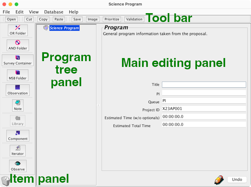
• Take a moment to acquaint yourself with the Observing Tool interface. You will find:

  • At the top: a tool bar with common actions.
  • On the left: a panel of items which you can add to your program.
  • In the center: a panel showing a “tree” view of your program.
  • The main editing panel occupying the remainder of the window.
  

• Fill in the program information for the top level “Science Program” item.

  Title

  A title for the program — usually the same as the proposal title.

  PI

  The project principal investigator. Enter your name here for this example.

  Queue

  You can just enter “PI” here for the EAO PI science queue — this field is not important.

  Project ID

  You can use a dummy ID such as X23AP001 for this example. When you store a science program to the OMP database, this ID is used to identify the project to which it belongs.

• Open the ACSIS library.

  • Select “File → Open ACSIS library” from the menu.

  Another Observing Tool window will open containing the library of sample ACSIS observations, organized in a series of folders based on the type of observation. The observations are each contained in a structure called an MSB (minimum schedulable block). An MSB is the basic unit used to schedule observing time within a night at the JCMT. Everything within an MSB must be observable, and all its constraints met, for us to select it to be done at any point in the night.

  You can expand each item in the library to browse the MSBs and the structure within them.

• Select the “Position-switch raster offset” MSB (blue cube icon) from the “Rasters — Classical” folder and copy it to your new science program using the “Copy” and “Paste” buttons in the tool bar.

• Expand each item in the tree panel of your new science program so that you can see the whole structure of the MSB.

• Now you can go through the MSB and customize each item to your liking.

  Note

  This note (shown in blue and with the “show to the observer” box checked) will be shown to the telescope operator when they perform the observation. You can include any information you wish them to be aware of regarding your program.

  Site quality

  Here you can choose “allocated” weather band and your observation will automatically be observed in any of the weather conditions approved by the time allocation committee for your project. It is also possible to further constrain the weather conditions by entering minimum and maximum opacity values (225 GHz, at zenith, labeled ‘τ’). Finally you can enter an opacity value to be used to compute noise estimates.

  Het Setup (HARP)

  This component selects HARP as the instrument we wish to use. We will return to this component later. For now, you can keep the default settings: 1 spectral region, 250MHz bandwidth mode and the CO 3–2 line.

  DR recipe

  This component allows you to select the data reduction recipe which will be used to process your data. The selected recipe name will be written to a FITS header in raw data files. It is used by ORAC-DR for on-line reduction in the summit pipeline, in the reductions performed for the JCMT archive (at CADC) and as the default recipe when you run ORAC-DR manually. Since our example MSB is a type of scan observation, select the recipe you wish to use (e.g. “REDUCE_SCIENCE_GRADIENT”) and press the “Set” button next to “Scan” to choose it.

  Target information

  Enter the following information at the top of this panel:

  • Name: NGC1333
  • Ra: 3:29:00
  • Dec: 31:15:00
  • Velocity: 15

  You will see that the information you have entered appears in the table below for the SCIENCE position. For this observation we will need also to specify a REFERENCE position. Since we copied an example raster MSB from the library, the REFERENCE line is already present, otherwise we could add it using the “Add” menu at the lower right. Select the REFERENCE line in the table and then enter the following information:

  • Offset: check box — you will see the Ra and Dec change to offsets in arcseconds.
  • Ra (offset): 0
  • Dec (offset): 300

  Science observation

  This sets up an observation which is to be performed as part of the MSB. In this example, the MSB only has one observation. Note that this panel shows an estimate of the time taken to perform the observation. Each observation will always have a “Sequence” containing one or more actual observe actions.

  Repeat (1X)

  This iterator would allow us to include multiple repeats of our map within the MSB. Leave this set to one repeat.

  Offset

  This iterator can be used to center the map at a position offset from the defined coordinates. It is also possible to specify multiple sets of offsets, in which case the observation will be repeated at each position listed. For now leave this component with the default offsets of (0, 0) arcseconds.

  Scan

  This type of item (with an eye logo) triggers the telescope to do something. In this case, we are requesting a scan of an area of the sky. Note that the scan strategy “Boustrophedon” is already selected — this corresponds to scanning back and forth across a rectangular area.

• If you want to keep your work, you can save the science program to an XML file on your computer.

  • Select “File → Save As…” from the menu.

  If this were a real observing program, you would want to store the program in our database rather than (or as well as) saving it on your computer. In that case, the telescope systems make automatic updates to your program, such as indicating when MSBs have been observed, so it is important to always start by fetching the current version from our database rather than opening an old file you may have saved previously.

Science Program settings are valid.

The position editor

We can use the position editor to visualize the observations in an Observing Tool program. This can be useful on its own, for example to verify that offsets and angles are being applied in the direction intended, but it is even more useful if you can load a reference image. We can convert one of the maps of NGC 1333 made in the data reduction tutorial to FITS format using the Starlink convert package, for example:

convert
ndf2fits \
    ../tutorial_prp/reduced-scuba2-pca/s20151222_00018_850_reduced \
    ngc1333.fits \
    comp=D bitpix=-32 encoding=FITS-IRAF \
    proexts=no prohis=no

Note that the “JSky” software used for the position editor only supports certain types of FITS files. The command above is based on the Observing Tool documentation, with the addition of proexts and prohis options to ensure extensions and history are not included (to reduce the FITS file size). In addition only certain projections, such as TAN, are supported correctly. The headers indicate that our file has this projection:

CTYPE1  = 'RA---TAN'           / Type of co-ordinate on axis 1
CTYPE2  = 'DEC--TAN'           / Type of co-ordinate on axis 2

If you do not have a map available to convert, please use the ngc1333.fits file in the section_1 directory.

We can display our FITS file into the Observing Tool's position editor as follows:

• Select the “Target Information” component in the program tree.

• Open the position editor window. There are three ways you can do this:

  • Click the “Image” button on the tool bar.
  • Select “View → Show the Position Editor” from the menu.
  • Click the “Plot…” button at the lower left corner of the main editing panel.

• Load our FITS file. This can be done in one of the following ways:

  • Click the open button in the tool bar.
  • Select “File → Open” from the menu.

• Adjust the color cut levels so that you can see the structure in the image. You can open the cut level window in either of these ways:

  • Click the cut levels icon in the tool bar.
  • Select “View → Cut Levels” from the menu.

  Adjust the levels so that you can see more of the structure: the automatic 98% setting may work well for this image.

• The position editor draws features related to the observations in pale colors. These can be easier to see with a plainer image color scheme. You can change the color scheme as follows:

  • Select “View → Colors” from the menu.
  • Choose a simple color scheme such as “Red” or “Blue”.

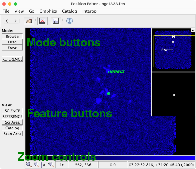
• Now let's take note of controls which are available in the panel at the left of the window:

  Mode buttons

  It is recommended that you use the tool only to visualize observations as you create them in the Observing Tool, keeping the “Browse” mode selected.

  Feature buttons

  As you select different components in your science program, different features will be available for plotting. Here you can select which of these features are drawn. Ensure that the “SCIENCE” and “REFERENCE” positions are enabled.

  

• You may immediately notice that there is a problem with our observation — there is emission at the reference position! (At least in the continuum as observed with SCUBA-2.)

  Return to the main science program window and try adjusting the reference position to move it away from areas of detection. The features in the position editor should automatically update to reflect your changes.

• You can enable the “Sci Area” feature to show the approximate field of view of the instrument (HARP).

• Now select the “Scan” eye in the program tree. In the position editor you should find a new feature button labeled “Scan Area”. Click this button to see the area defined by our scan pattern. (It is best to also disable the “Sci Area” feature here so that only one area is shown.)

  We can adjust the size of the scan area and see the result in the position editor:

  • You may notice that if you select the MSB or the observation, the estimated time is 26 minutes.
  • In the scan component, increase the width and height to 360 arc-seconds.
  • You should see the increased size reflected in the position editor.
  • However, looking at the MSB or observation, the time estimate will have increased to 73 minutes.
  • We can reduce the time to something more reasonable by decreasing the “Sample Time” in the scan eye, perhaps to 2 seconds. This would cause the telescope to scan more quickly.

  By enabling the “REFERENCE” feature, we can check that the reference is not inside the scan area.

• Finally select the “Offset” iterator in the program tree and ensure the “Offset” feature is enabled in the position editor. You should see a point (plotted as a yellow circle) labeled 0 (meaning this is offset number zero).

  We can adjust the offset values to try to center our scan on the emission detected by SCUBA-2. Offsets of about p=30, q=-30 should achieve this. (In this configuration, p will be RA and q will be declination.)

  Warning: If you now select the “Scan” eye in the tree, you will see that the position editor shows the scan in the original, non-offset position. This illustrates an important point about the position editor: it plots information about the selected component. Therefore to see the offset position, we must select the offset iterator.

Survey containers

Survey containers allow you to repeat an MSB for multiple targets. In this example we will place a SCUBA-2 daisy observation in a survey container and load a target list from a file.

If you have the latest version of Starlink installed, you will be able to use the catalog_convert script to convert a target list downloaded from Hedwig to the Observing Tool survey container format. If you have a proposal in the Hedwig system, you can download a target list using the link under the table in the Target Objects section of the proposal. Alternatively use the example in the section_1 directory of the tutorial package. You can perform the conversion as follows:

catalog_convert --infmt hedwig --outfmt jcmt_ot_sc \
    section_1/targets.txt survey_container.txt

This should give:

SCIENCE NGC1333 03:28:54.000 31:16:52.00 FK5 -1 1 1
SCIENCE IC348 03:44:18.000 32:04:59.00 FK5 -1 1 1
SCIENCE NGC2024 05:41:41.000 -01:53:51.00 FK5 -1 1 1
SCIENCE NGC2068 05:46:13.000 -00:06:05.00 FK5 -1 1 1

Each line either defines a SCIENCE or REFERENCE position. Then following the name and coordinates are three numbers: position in tile (-1 for JCMT), number of repeats and priority. More information on the format of this file is available on the Observing Tool advanced topics page.

If you do not have the catalog_convert script available you can use the survey_container.txt file in the section_1 directory.

You can set up the survey container as follows:

• Select the top-level science program entry in the program tree panel. This will ensure that the Observing Tool does not try to insert the survey container inside our existing MSB.

• Add a survey container to the program by clicking the “Survey Container” button in the item panel at the left of the window.

• Open the SCUBA-2 library:

  • Select “File → Open SCUBA2 library” from the menu.

• Copy the daisy map MSB into the survey container:

  • Open the “Pointsource (Daisy)” folder, select the “Pointsource Daisy map” MSB and copy it using the “Copy” button in the tool bar.
  • Return to your science program window, ensure the survey container is selected and click the “Paste” button in the tool bar.

• Open all of the components in the daisy map MSB so that you can see everything. You may notice that the example from the library includes a “Target Information” component, but this is not required since we will be specifying targets through the survey container. In fact, if you trying validating the science program at this point, you will see an error:

  ERROR: An MSB within a Survey Container may not contain a Target Component
  

  • Select the “Target Information” component in the daisy MSB and delete it using the “Cut” button in the tool bar.

• Select the observation item and note the estimated time of 31 minutes — this is the 1800 second integration time from the “Scan” eye plus some allowance for observing overheads.

• Next we will set up the target list in the survey container itself:

  • Begin by selecting the “Survey Container” entry in the program tree panel.
  • Click the “Load” button at the bottom of the panel and open the survey_container.txt file we prepared earlier.
  • The initial default position of 0:00:00 0:00:00 will still be present at the top of the survey container. Select this entry and click the “Remove” button to delete it.

  Note how the observations remaining counter values and priorities have also been loaded from the text file. You can alter these values by selecting a target and using the controls at the bottom of the panel.

• It is also possible to edit survey container targets directly in the Observing Tool. You can do this by selecting one of the targets and then clicking the “Target Information” tab at the top of the panel. This opens a similar interface to that used to configure an individual target. Targets can have reference positions here when necessary. Click the “Survey Targets” tab to return to the list.

• Finally select the MSB item in the program tree and check the estimated time. Even though we have multiple targets, the time to perform the MSB should be 31 minutes — the same as the observation inside.

  If instead we had set this program up with the survey container inside the MSB, that would indicate that everything had to be done in a single session. If the science program is arranged in this manner you will find that the time for the MSB becomes excessive. This is clearly not what we want in this case!

  If you select the top level science program entry in the tree panel, you can check the total time for the whole program. This will change depending on the number of targets, but with the example given here, it might be about 2 hours 40 minutes — this is 4 × 30 minute SCUBA-2 daisy maps, plus 40 minutes for the HARP raster MSB.

The frequency editor

Next we will create a heterodyne setup to observe the following lines simultaneously with ʻŪʻū:

1. CO 2–1 (USB)
2. ¹³CO 2–1 (LSB)
3. C¹⁸O 2–1 (LSB)
4. N₂D⁺ 3–2 (USB)

You can do this as follows:

• Open the ACSIS library and copy the “Beam-switch stare” MSB to your program.

• Open all parts of the new MSB. You can fill in the target information component and select a DR recipe for “stare” mode.

• Select the “Het Setup (HARP)” component in the tree panel and change the front end to “Uu”. Dialog boxes may pop up to indicate adjustments which the Observing Tool is making to the tuning information. You will then see that the name of the component in the tree has changed to “Het Setup (Uu)”.

• Now you can complete the front end configuration:

  Sp. Regions

  Change to 4 because we wish to tune 4 separate lines. Again dialog boxes may pop up as the Observing Tool makes adjustments.

  Mode

  “2sb” will be the only option. This is a sideband-separating receiver — we can set up lines in both sidebands and they will generate separate subsystems in the raw data. In addition spectra will be recorded in the image frequency of each tuned line.

  Sideband

  Since our first line is in USB, select “usb” here. Note: we cannot use “best” because we will be setting up lines in both sidebands — we need to specify exactly which line will be in which sideband.

• CO 2–1 may already be selected in the frequency setup panel. If not, select it from the menu boxes.

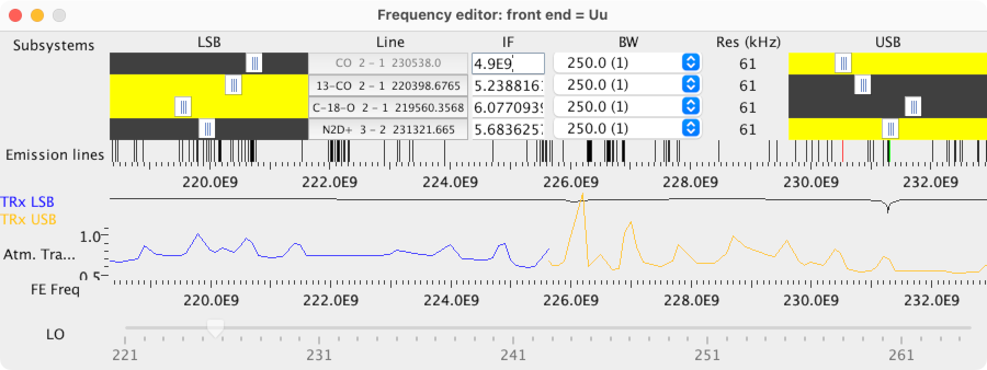
• Open the frequency editor by clicking the “Show Frequency Editor” button. You should see that the editor has:

  • 4 subsystems indicating the selected IF frequency. This frequency is also shown by the sliders for the LSB and USB sidebands. The slider for the selected sideband will be highlighted in yellow.
  • A plot of the locations of emission lines from the Observing Tool’s catalog. The positions of these lines corresponds to the sliders for the subsystem IF frequencies.
  • Graphs of the receiver temperature and atmospheric transmission. Again these correspond to the position of the IF frequency sliders.

• The overall tuning is controlled by the first subsystem. This will already be set to CO 2–1 but we need to lower the IF frequency to fit all of the intended lines. Change the IF of the first subsystem to 4.9E9. You will see that the other subsystems now show “No Line” since they are no longer tuned to the original line.

• Next choose 13-CO for the 2nd subsystem: right click on the emission lines below the LSB sliders. A pop up menu will show lines close to where you clicked. Choose “13-CO 2 - 1” from the menu then click on the “Line” button for the 2nd subsystem (currently labeled “No Line”). You should see that the LSB slider becomes highlighted and the relevant IF frequency is filled in.

• Choose “C-18-O 2 - 1” for the 3rd subsystem in the same way.

• Choose “N2D+ 3 - 2” for the 4th subsystem. Since this is in the USB range, you will need to open the menu from around the middle of the USB slider.

  

• Finally save the selected configuration into the Observing Tool by clicking the “Hide Frequency Editor” button in the “Het Setup” panel. Alternatively close the frequency editor window and click “Yes” in the dialog box which appears.

Completed example

If you would like a completed example of the science program described here, please see the file program.xml in the section_1 directory.

2. Organizing programs

In this section we will see two quick ways in which you can improve the organization of a science program in the Observing Tool.

Inheritance

This example features a simple but very repetitive science program. The aim is simplify the program by reducing the amount of duplicate information.

• Open the inheritance.xml file from the section_2 directory.

• Take a look through the structure of this science program. You should notice that:

  • Each MSB has a different target and scan parameters.
  • Everything else is exactly the same in each MSB.

• Remember that when an item is present at one level in a science program tree, it applies to everything at lower levels. So we can move the common items to the top level rather than duplicating them in each MSB.

  There are two ways you can move an item:

  • Cut the item and then paste it into its new location using the “Cut” and “Paste” buttons in the tool bar.
  • Drag the item to its new location.

  If you choose to move an item by dragging it, you will notice the icon of the target location change as follows:

  Down-pointing arrow

  The item will be moved below the target location.

  Diagonal downwards arrow

  The item will be moved inside the target location. If instead you wished to move it below the target, move the pointer further to the left.

  Red circle with ×-mark

  This indicates that the item can not be moved here.

  Go ahead and move the “SCUBA-2” item to the top level of the program, just above the first MSB.

• Now that you have SCUBA-2 at the top level, you don't need to repeat it in all the other MSBs. Select this item in each MSB and use the “Cut” button in the tool bar to remove it.

• You can repeat this procedure for the other duplicate items, such as the notes and the “Site Quality” and “DRRecipe” components.

• Imagine that you want to add something special to the notes for just one of the MSBs. Initially this might seem a problem, since we have a single note for all of them!

  However the OMP will combine multiple notes when someone views your MSBs. Therefore we can simply add a new note to one of the MSBs and put just the extra information there.

  Try adding an extra note to one of the MSBs. Don’t forget to check the “Show to the Observer” box so that the note is shown to the operator at the telescope.

If you would like to compare your science program with a completed example, please see the file inheritance_completed.xml in the section_2 directory.

“And” folders

“And” folders are used to group a collection of MSBs together. The most common uses for them are organizing a program and applying common settings to a number of MSBs. When used in these ways, “and” folders do not affect the observation of MSBs inside — they are still each done individually.

• Open the and_folders.xml file from the section_2 directory. This is a science program containing a few MSBs based on the JCMT calibration program’s spectral line standards for HARP.

• Note how several common items are located at the top level so that they apply to all MSBs:

  • Note
  • “Site Quality” component

  However the targets, receiver tuning information and in some cases observing mode differ between the MSBs. Also the “DRRecipe” components are placed next to the “Het Setup” components because the Observing Tool needs to know which instrument is being used when configuring DR recipe choices.

• We can organize this program by making an “and” folder for each molecular line being observed.

  • Select the “Site Quality” component — just above the first MSB — since we should add folders here.
  • Click the “AND Folder” button in the item panel twice to add two folders to the program.
  • Select each of the new folders in turn and edit their titles. Since we will be using one for each molecular line, you could call them “C18O standards” and “HCN standards”.

• Move each MSB to the corresponding folder. You can do this either by dragging them and dropping them inside, or by cutting and pasting them.

  You should end up with the two C¹⁸O 3–2 MSBs in one folder and the two HCN 4–3 MSBs in the other.

  The science program is already more organized than it was before. If the program had a large number of MSBs, then the ability to open and close folders as a whole would be very useful. Note that making this change does not alter how the program will be observed — each MSB is still observed individually.

• Finally we can use inheritance to avoid having duplicate tuning information for each set of MSBs:

  • Move the “Het Setup” component from the first of the C¹⁸O MSBs to the top of the folder.
  • Remove the duplicate “Het Setup” component from the second of the C¹⁸O MSBs.
  • Repeat the process for the HCN MSBs, so that you only have one copy of the “Het Setup” component at the top of the folder.
  • You can do the same for the “DRRecipe” components, placing them just below the corresponding “Het Setup” components.

A completed copy of this example can be found in the and_folders_completed.xml file in the section_2 directory.

3. The validator

This example is intended to allow you to practice working through the output of the Observing Tool’s validation tool. A science program with a number of intentional errors is provided.

• Open the validation.xml file from the section_3 directory.

• Select one of the MSBs in the program and press the “Validation” button in the window toolbar.

  Note how the Observing Tool shows just the internal check results for the selected MSB.

• Select the main science program item (labeled “Problematic Program”) and press the “Validation” button.

  Note now the Observing Tool now shows internal check results for all MSBs and the XML schema validation results.

• Try to adjust the program to correct the problems identified by the validator.

  We recommend that you work on one MSB at a time, validating that individual MSB. Afterwards you should validate the program as a whole.

• Can you see any more problems with this program that the validator does not find?

Once you have finished correcting the science program, please take a look at the list of additional problems in the issues.html file in the section_3 directory. You can also compare your program with the validation_completed.xml file.