


The ACSIS digital autocorrelation spectrometer is used as the backend for the spectral line receivers.
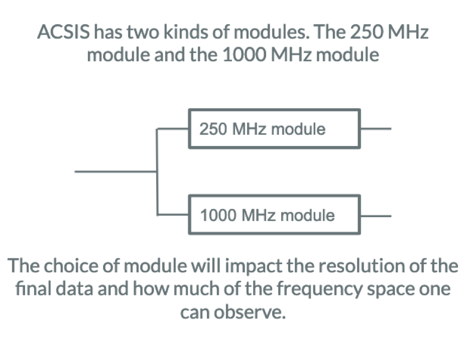
The ACSIS (Auto Correlation Spectral Imaging System) digital autocorrelation spectrometer is used as the backend for the spectral line receivers HARP, RxA, RxW, and Nāmakanui. ACSIS have a maximum of 4 DCMs/correlators fed from the same IF. ACSIS can therefore be configured with up to two (HARP) or four (Nāmakanui) spectral windows and supports a variety of bandwidth modes ranging from 250 to 3200 MHz. The spectral resolution of ACSIS varies from 30 kHz to ~1 MHz, depending on the configuration used.
To support fast mapping of large areas the data can be read out at a rate of 0.1s. This allows large areas to be scanned rapidly.
Contents
Available Bandwidth Modes
ACSIS has in total 32 down converter modules (DCMs) and correlator cards. A DCM “picks out” a 250 or 1000 MHz wide subband from an IF input and feeds the signal to a correlator card. Note a maximum of 4 DCMs/correlators fed from the same IF. HARP has 16 IF outputs, and Nāmakanui has 4 IF outputs (4 for ʻŪʻū at 230 GHz and 4 for ʻĀweoweo at 350 GHz), while there are 32 DCMs and correlator cards. The “excess” of DCMs and correlator cards can be used in two ways, e.g. for HARP:
- Chaining two correlator cards together doubling the number of channels in a 250 or 1000 MHz subband.
- Use two DCMs to extract two frequency subbands from each of the 16 IF inputs and feed each subband to a correlator card. This creates two spectral windows to follow the OT terminology. (*see footnote below)
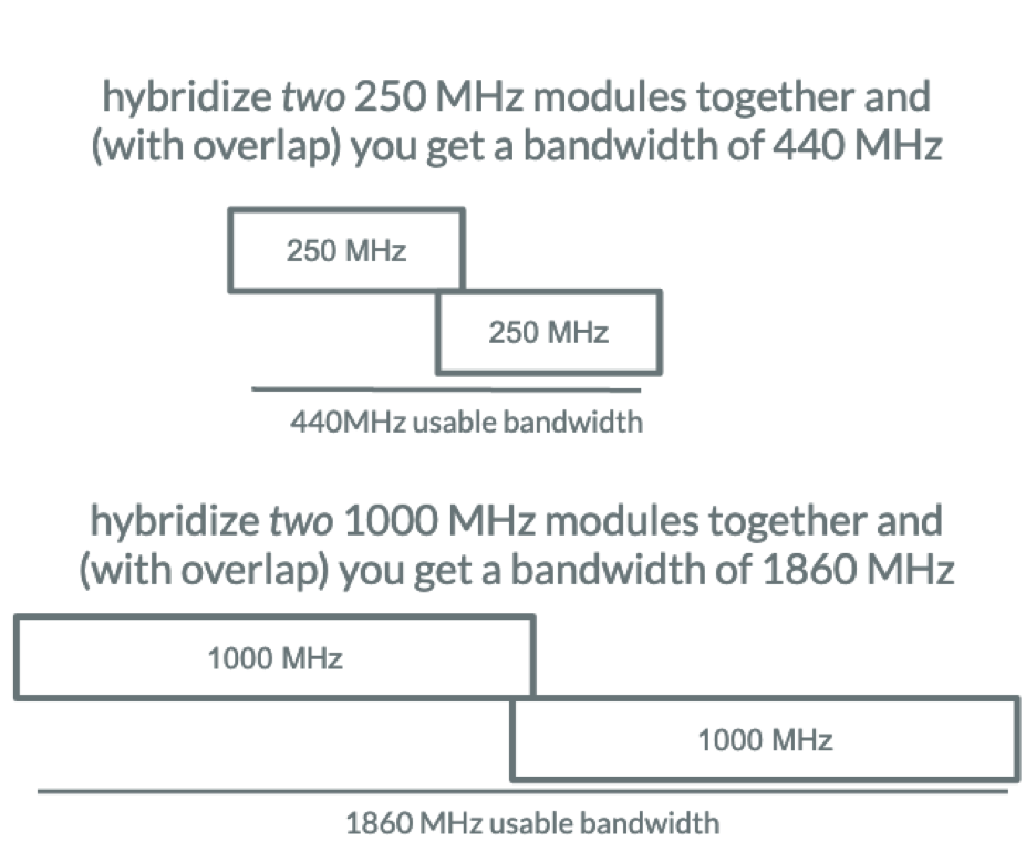
Hybrid mode: The OT supports a special case of option two – by changing the selection of numbers of spectral regions, the OT automatically use the 250 and 1000 MHz modules to produce a variety of bandwidth modes from 400 to 3200 MHz (this also depends on the IF range of certain receiver) with subbands overlap slightly. These subbands can be merged later in the data reduction. New options such as the 1600 and 1800 MHz bandwidths have a larger overlap between the two subbands (but the same spectral resolution) than the 1860MHz bandwidth. This is useful when the spectra contain very broad lines. Caution: due to the subband overlap which might cause baseline issues, using hybrid wideband mode is only advised when absolutely necessary, for example, used for the Galactic Centre with its large velocity range, galaxies with significant velocity dispersion (> 600 km/s), or spectral line surveys.
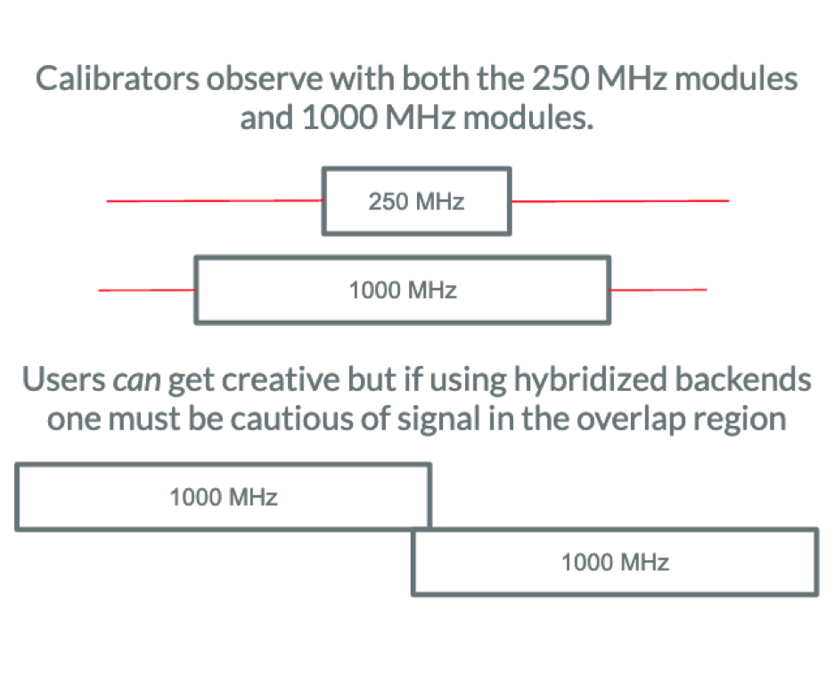
Note (a): the merging used to be done by the ACSIS DR system – for further details see note (b). Also, when using 440 or 1860 MHz bandwidth it might be better not to place the line in the center when using hybrid modes – since that places the line in the overlap region (see section 1.4).
Note (b): The merging in the ACSIS DR occasionally created artificial features where the spectra were joined. The reason was too small overlaps and that the merge was weighted by the total power drop off. In principle, Tsys weighting would be better but the estimated Tsys also gets very uncertain at the edge. Further, merging the spectra was an irreversible process. Thus, if there was a problem we could not go back and reprocess the data. Therefore we do now store the unmerged raw spectra and the merging is done in the post-processing.
An example of the second use is to observe 13CO 3-2 and C18O 3-2 using two spectral regions (subbands). A number of such setups are pre-prepared and can be selected as “spectral configurations” in the OT. They are listed at the bottom of this page.
An example of the hybrid mode is to select 1860 MHz mode for an extragalactic source with a broad line. In this case, it is less error-prone to let the OT do the setup than “manually” do the setup using the frequency editor. Further, it has the advantage that data from both spectral regions will record the same rest frequency.
(*) All 32 DCMS are used in either case. While correlators of typical design would chain correlator cards together ACSIS has a different design. In this mode each IF uses two DCMs each connected to a single correlator card. The two independent systems are time-interleaved – they record data for half of the time each and replay it all the time. The slower replaying speed allows the increased number of resolution channels. Afterward, the two independent spectra are averaged in the software.
HARP
HARP has 16 IF outputs while there are 32 DCMs and correlator cards. The spectral window and bandwidth possibilities for HARP are summarized in the table below.
| Spectral windows |
Bandwidth mode | Channel Spacing | Usable Bandwidth | Channels | Number of DCMs |
| 1 | 250 | 0.0305MHz | ~220MHz | 8192 | 2 |
| 1000 | 0.488MHz | ~930MHz | 2048 | 2 | |
| 1860 (1600, 1800) | 0.977MHz | ~1860(1600,1800)MHz | 1904 (1638, 1843) | 2 | |
| 440 (400, 420) | 0.061MHz | ~440(400,420)MHz | 7208 (6563, 6881) | 2 | |
| 2 | A 250 | 0.061MHz | ~220MHz | 4096 | 1 |
| 1000 | 0.977MHz | ~930MHz | 1024 | 1 |
E.g. if two spectral windows are selected in the OT one with a bandwidth of 250 MHz and the other with a bandwidth of 1000 MHz, the result is one spectrum of usable bandwidth ~220 MHz and channel separation 61.0kHz and one spectrum with usable bandwidth ~930 MHz and channel separation 0.977 MHz. Also note that if the 1860 or 440 MHz option is selected only one spectral window is allowed – the 32 DCMs and correlator cards have already been used up! As can be seen from channel spacing in the table the 1860 and 440MHz modes are using two subbands. Conversely, if you select two subbands only the bandwidth options 250 and 1000MHz exist.
Nāmakanui (& RxA)
RxA was not able to use all the DCMs and correlator boards in ACSIS – see the HARP section. For Nāmakanui, a maximum of 4 DCMs/correlators can be fed from the same IF in a usable way. Thus, one can select 1 – 4 spectral windows for each IF output with the bandwidth mode summarized in the table below.
| Spectral windows | Bandwidth mode | Channel Spacing | Usable Bandwidth | Channels | Number of DCMs |
| 1 | any 250 | 0.0305MHz | ~220MHz | 8192 | 2 |
| any 1000 | 0.488MHz | ~930MHz | 2048 | 2 | |
| any 440(a) | 0.0305MHz | ~440MHz | 14417 | 4 | |
| any 1860(b) | 0.488MHz | ~1860MHz | 3809 | 4 | |
| 2 | A 250 or 1000 MHz spectral window above, AND | 0.0305MHz | ~220MHz | 8192 | 2 |
| any 1000 | 0.488MHz | ~930MHz | 2048 | 2 | |
| any 440(b) | 0.061MHz | ~440MHz | 7208 | 2 | |
| any 1860(b) | 0.977MHz | ~1860MHz | 1904 | 2 | |
| 3 | A spectral window as in one of the four rows above (c) | 2 | |||
| any other 250 | 0.061MHz | ~220MHz | 4096 | 1 | |
| any other 1000 | 0.977MHz | ~930MHz | 1024 | 1 | |
| 4 | any 250 | 0.061MHz | ~220MHz | 4096 | 1 |
| any 1000 | 0.977MHz | ~930MHz | 1024 | 1 |
Note: (a) with one spectral window, hybrid modes of 400, 420, 440, 600, 800, 1600, 1800, 1860, 2400, and 3200 MHz are provided automatically in the OT by combining several 250 or 1000 MHz modules together.
(b) with two spectral windows, hybrid modes of 400, 420, 440, 600, 1600, 1800, 1860, and 2400 MHz are supported automatically (resolution might be different from one-spectral-window).
(c) with three spectral windows, hybrid modes of 400, 420, 440, 1600, 1800, 1860 MHz are provided automatically in the OT.
For the curious – with 3 spectral windows and 4 DCMs/correlator cards the DCMs/correlator cards can only be distributed 1+1+2 over the three spectral windows. The spectral window with 2 DCMs/correlator cards can support higher resolution or higher bandwidth.
Diagrams of spectral windows
A note on hybride modes
It should be noted that hybride modes like 400, 440, 1600, etc are implemented purely in software and does not involves the receiver or ACSIS. The translator sets up the LO2s so the DCMs spectral range overlaps and ORACDR combines the data from the spectral ranges that overlaps. From an ACSIS point of view there observations remain a set of 250 or 1000 MHz configured DCMs with a set of LO2s.
ACSIS does not do anything different if these spectral windows overlap or not. The receiver itself only cares about the frequency and Doppler correction to tune the receiver as needed.
ACSIS Special Configurations
The table below describes the ACSIS special configurations which are available within the Het Setup component of the Observing Tool (OT). If the special configuration you require is not among the list below (or in the OT), you may create your own configuration using the Frequency Editor tool. However, we strongly urge you to send a request to helpdesk@eaobservaotry.org so that we can add the new configuration to the list.
Name		   Receiver  Systems Mode   Sideband  Species   transitions     Bandwidths

RxA_H2CO_250X3	     A3		3    DSB      LSB	H2CO	3 0 3 - 2 0 2		250
							H2CO	3 2 2 - 2 2 1		250
							H2CO	3 2 1 - 2 2 0		250

RxA_13C18O_250X4     A3		4    DSB      USB	13-CO	2 - 1			250
							C-18-O	2 - 1			250
							SO	5 6 - 4 5		250
							SO	5 6 - 4 5	       1000

RxA_SIOSO_250x2	     A3         2    DSB      LSB	SiO	6 0 - 5 0		250
							SO	4 3 - 3 4	        250

RxA_SiO54_v12_250X2  A3         2    DSB      LSB       SiO     5 2 - 4 2               250
                                                        SiO     5 1 - 4 1               250

HARP_COH13CN_250    HARP        2    SSB      LSB	CO	3 - 2			250
							H-13-CN	4 - 3			250

HARP_H2DN2H_250X2   HARP        2    SSB      USB	H2D+	1 1 0 0 - 1 1 1 0	250
							N2H+	4 - 3			250

HARP_13C18O_250x2   HARP        2    SSB      LSB	C-18-O	3 - 2			250
                                                        13-CO   3 - 2                   250

HARP_DCN_HNC_250x2  HARP        2    SSB      best      DCN     5 - 4                   250
                                                        HNC     4 - 3                   250

HARP_CO_H13CO_250x2 HARP        2    SSB      best      CO      3 - 2                   250
                                                        H13CO   4 - 3                   250

HARP_C170_C34S_250x2 HARP	2    SSB      best	C-17-O	3 - 2			250
							C-34-S	7 - 6			250