Data & Software Blog: tips, tricks and new features

This is the Scientific Computing group’s blog. It hosts various posts highlighting new features, bug fixes and interesting tips for users of the JCMT and EAO’s software and data.

You can subscribe to notifications of all new posts in this blog by joining EAO’s software discussion mailing list. You can join either by going to this address, or by sending an email to software_discussion+subscribe@eaobservatory.org.

You can also use this mailing list to ask questions of both EAO’s Scientific Computing staff and your fellow JCMT users. It’s currently very low volume. One can search by tag by software on instrument:

starlinkSMURFHDS-v5makemap

ACSISHARP`Ū`ūSCUBA-2POL-2


Stardev Matched Filter Change

On July 1st, 2021 the two-component SCUBA-2 beam profile parameters were updated in accordance with the results published by Mairs et al 2021. This caused a change in the Matched Filter post-processing.

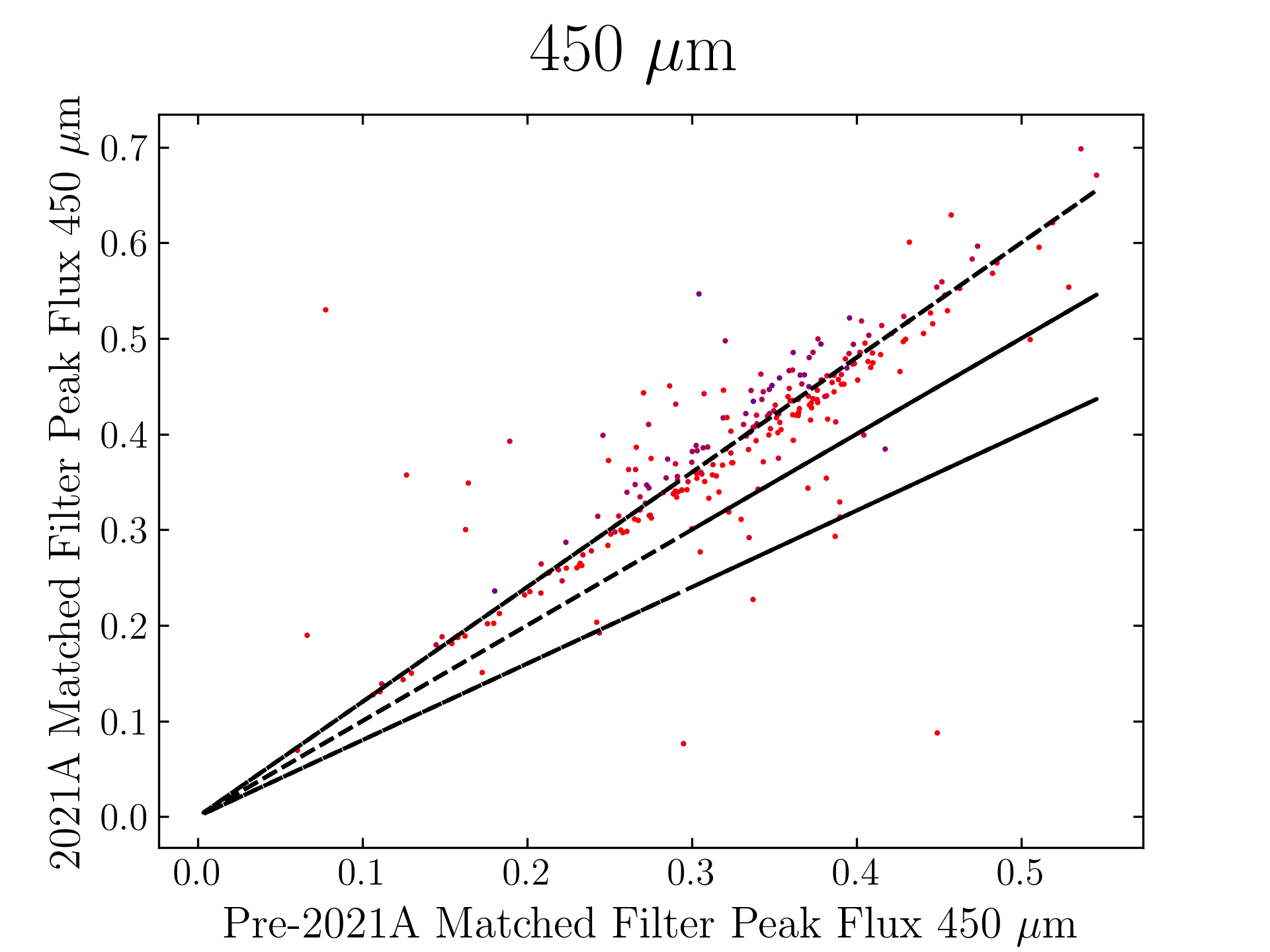
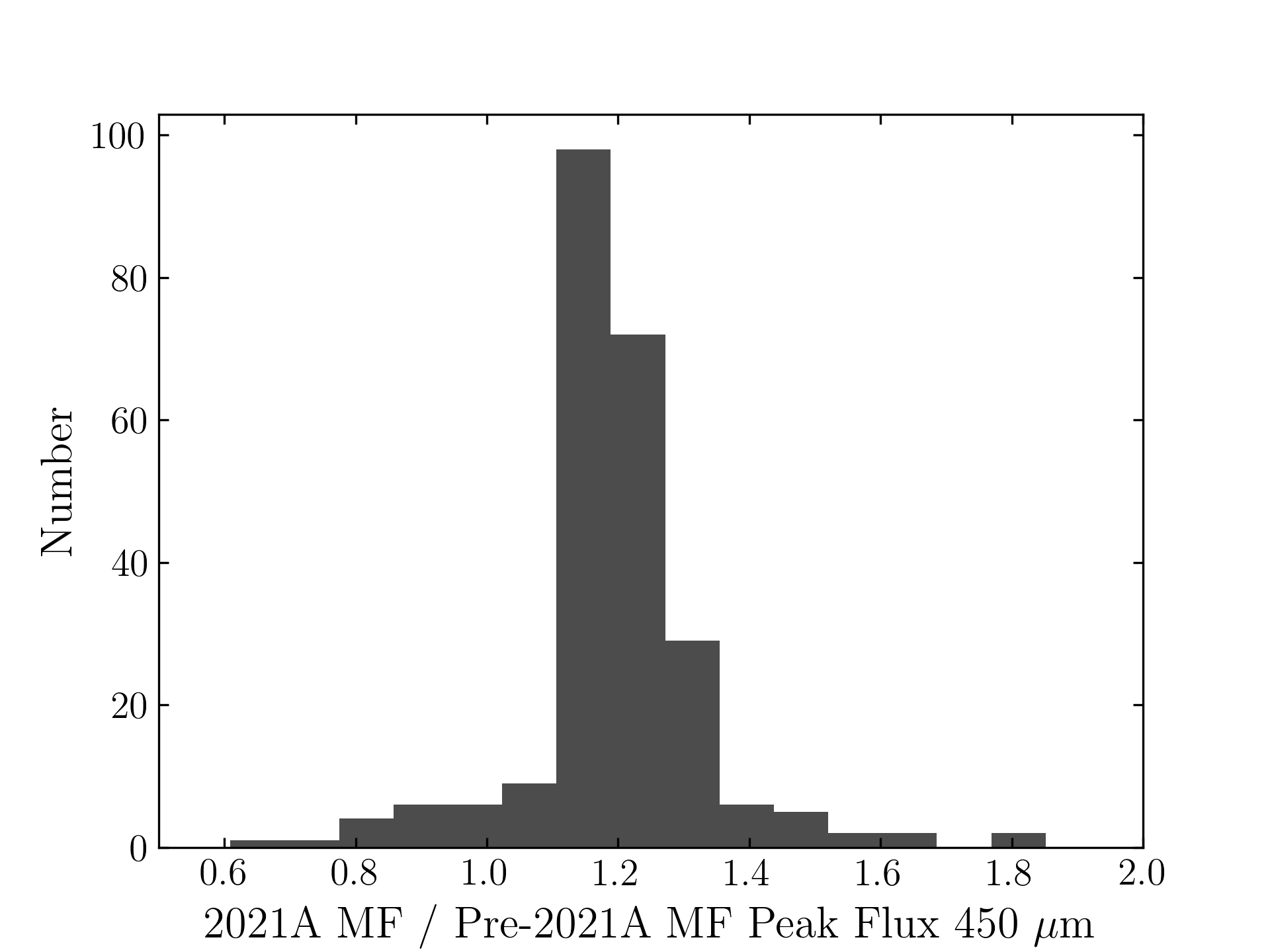
When using a Stardev installation post-July 1st, 2021, executing the matched-filter method is expected to increase the measured peak fluxes of bright point sources by ~15% relative to older versions of Starlink. A similar factor may apply to faint point sources in otherwise “blank fields” but this requires further testing.

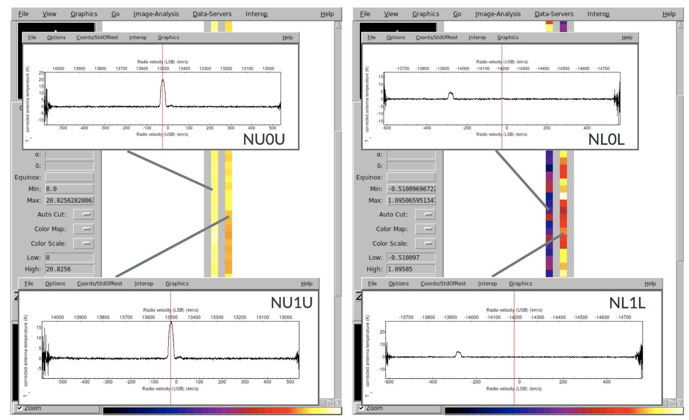
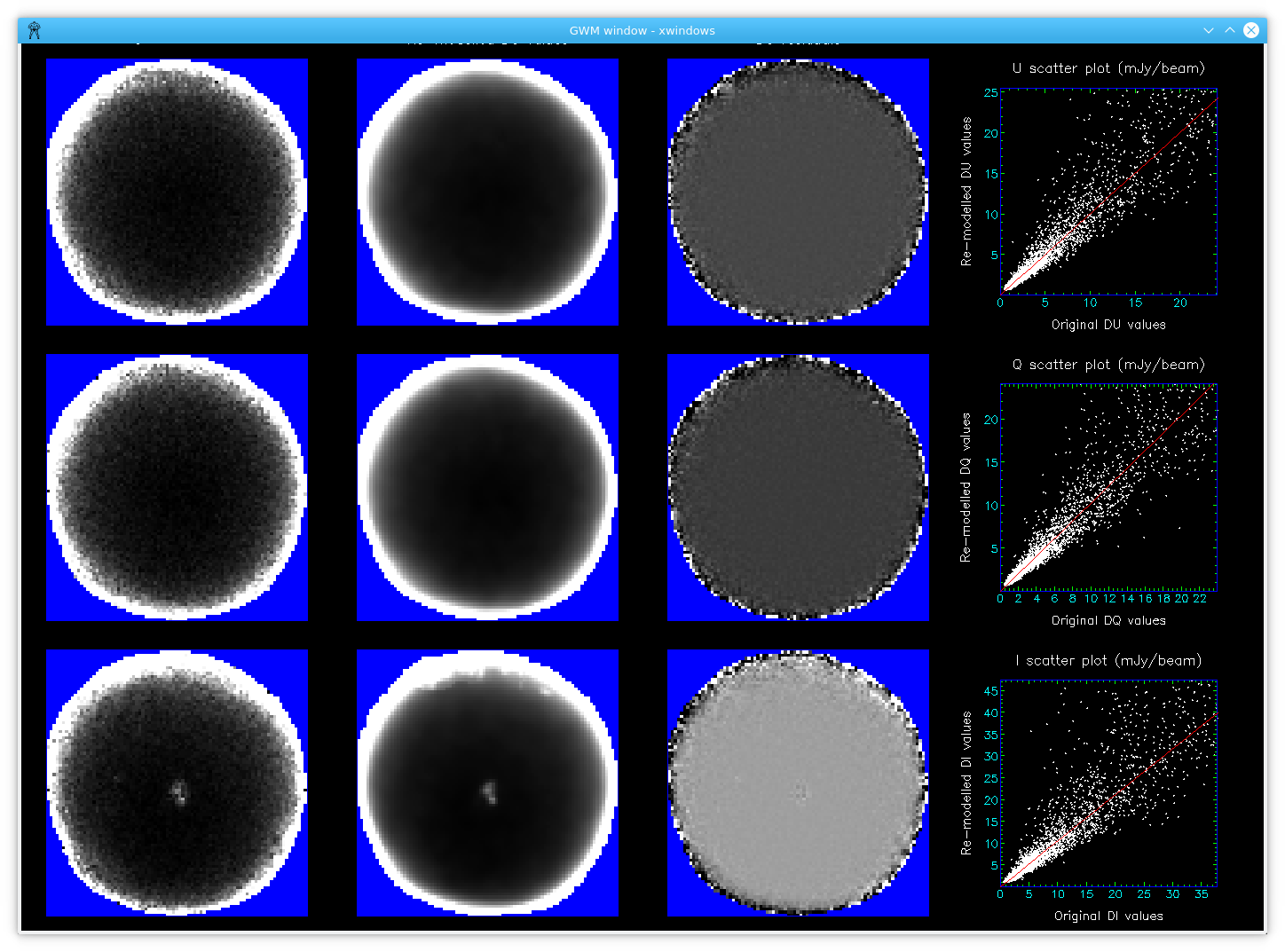
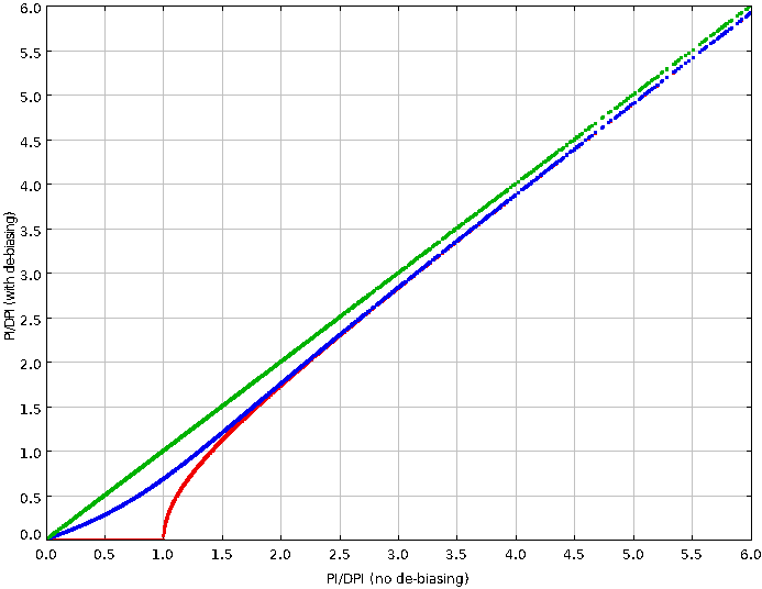
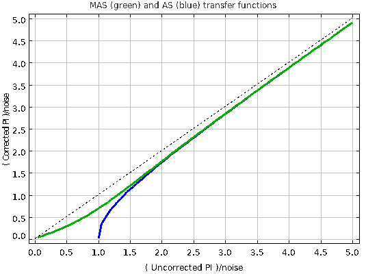
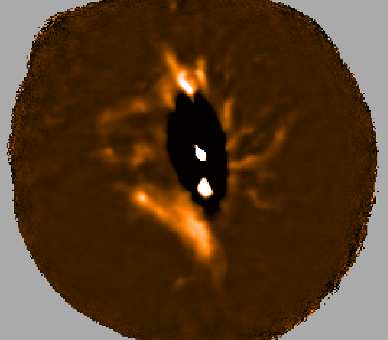
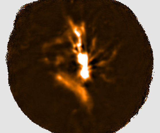
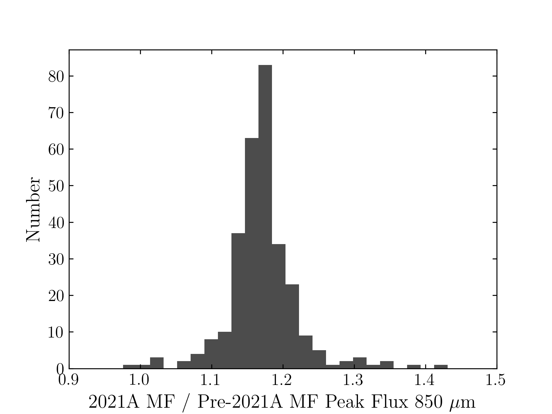
The plots, below, show comparisons between the 2018A Starlink and most recent Stardev matched filter implementation on Uranus calibrator observations taken between 2016-11-01 and 2021-04-13. Note that the Stardev version consistently returns peak flux values that are ~15-20% higher than before due to updated empirical beam measurements presented in Mairs et al 2021.

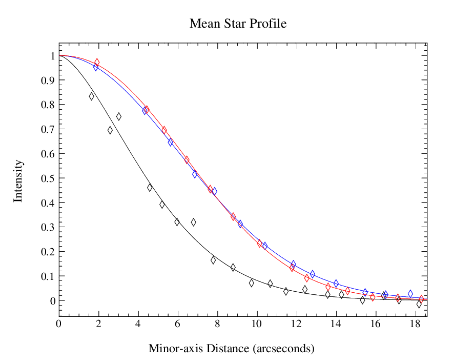
The beam patterns for matched filtering purposes are described as a combination of two Gaussian functions:

G_total = α*G_mb + β*G_sec,

where each Gaussian profile, G, is of the form exp[−4*ln(2)*(r/θ)^2], where “r” is the radial distance from the centre and θ is the FWHM of the profile, both measured in units of arcseconds. The first component, G_mb represents the “main beam” response. The second component, G_sec, is an approximation of the “secondary beam” or “error beam”, which describes the flux in the shoulders of the profile. α and β are coefficients describing the relative contribution of each component (the amplitudes). The broad error beam includes factors such as sidelobes due to diffraction, static dish deformations, and dish deformations induced by thermal gradients.

450 microns:

850 microns:

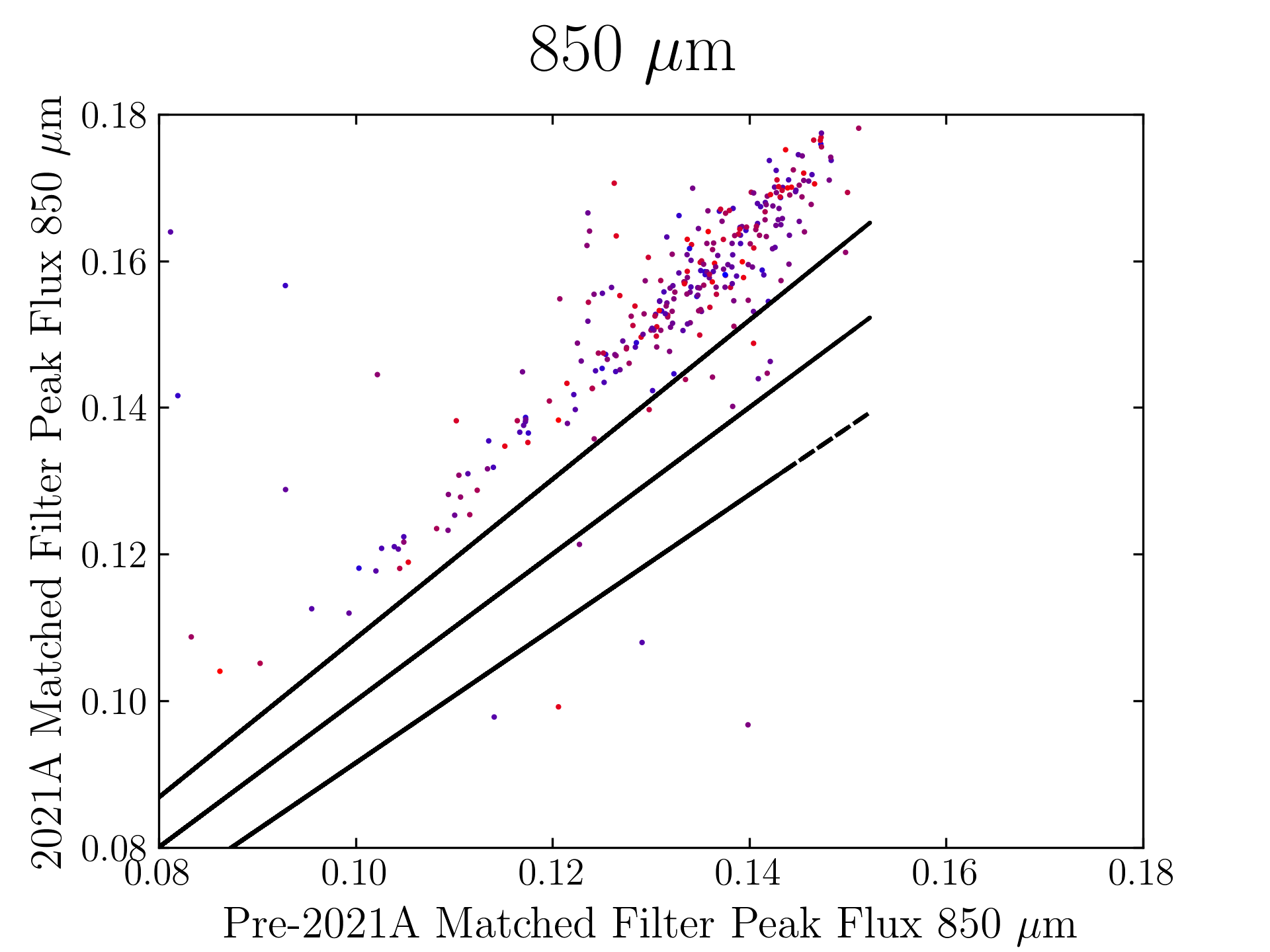
The original SCUBA-2 Beam Parameters were presented by Dempsey et al. 2013:

450 microns:

α = 0.94
β = 0.06
θ_mb = 7.9
θ_sec = 25.0

850 microns:

α = 0.98
β = 0.02
θ_mb = 13.0
θ_sec = 48.0

The updated SCUBA-2 Beam Parameters are presented by Mairs et al 2021:

450 microns:

α = 0.89
β = 0.11
θ_mb = 6.2
θ_sec = 18.8

850 microns:

α = 0.98
β = 0.02
θ_mb = 11.0
θ_sec = 49.1

These values represent the median results after fitting the two-component model to all Uranus calibrator observations since May, 2011 above a significant transmission threshold (see Mairs et al 2021).

The total area of each beam profile, A, can be calculated by:

A = {π/[4*ln(2)]}*[α*(θ_mb)^2+β*(θ_sec)^2].

Comparing the Dempsey et al 2013 beam areas to the Mairs et al 2021 beam areas reveals a ~20% difference at both wavelengths (in practice, there is a spread around this typical 20% value, see plots, above).

Note that previously, it has been common practice in cosmology publications employing “Blank Field” data reduction recipes (e.g. REDUCE_SCAN_FAINT_POINT_SOURCES, REDUCE_SCAN_FAINT_POINT_SOURCES_JACKKNIFE) to apply a correction factor of ~10% in order to compensate for flux lost due to filtering. This 10% factor was derived by inserting a bright Gaussian point source into the raw power versus time stream of individual observations and measuring the response of the model to the filtering during the data reduction process (e.g. Geach et al. 2013, Smail et al. 2014). We recommend repeating this experiment with the new Starlink 2021A matched-filter implementation for your specific data in order to determine whether the correction factor is still necessary.

KAPPA/POL2MAP bug causes incorrect variances and error values

A bug was introduced into the cmult and cdiv commands in the Starlink KAPPA package on 21st May 2021. This bug caused incorrect Variance values to be stored in the output and was fixed on 12th July 2021. Consequently, anyone who uses these commands and who last rsynced the nightly Starlink build from EAO between these dates should consider rsyncing the current nightly build, which includes the bug fix.

POL2 users should be aware that the cmult command is used within the pol2map script when converting values from pW to mJy/beam. This means that vector catalogues produced by pol2map will contain incorrect DI/DQ/DU values if starlink was rsynced between the two dates mentioned above.  Again, the solution is to rsync the current nightly build, which includes the bug fix.

Bug in POL2MAP

A  recent change in the Starlink KAPPA package causes the SMURF pol2map command to crash . The main symptom is a message at the end of the pol2map logfile that looks something like this:

+ -50
. could not convert string to float: '+ -50'

The change that causes this problem occurred on 30th April 2021 so will affect Starlink installations copied from EAO on or after that date. The problem has been fixed today (19th May) so anyone affected by this problem should copy starlink again after completion of the next nightly build.

Thanks to Jeremy Yang for reporting this problem.

ACSIS software update to track per-subsystem

On 20201202 we updated our ACSIS software. In the past all receptors would be written our to raw files on a per-observation basis. For the Nāmakanui insert `Ū`ū this meant that for each observation a minimum of two files would be produced, one for LSB and one for USB, each containing 4 receptors: NU0L, NU0U, NU1L, NU1U. This led to writing out blank data. Below is a quick reminder of Nāmakanui receptor naming convention:

  • N= Instrument: Nāmakanui
  • U = Insert: `Ū`ū
  • 0/1 = Polarization: 0/1
  • L/U = Side-band: LSB/USB

The ACSIS software update now keeps track of working receptors per-subsystem (spectral window) instead of per-observation, and thus does not write blank data to the .sdf output files for non-contributing receptors. This is mostly for the sake of Nāmakanui, but will also affect HARP regarding the order the receptors appear in the output files. Thus if you look at raw `Ū`ū  data files taken before the change you will see blank data.

Raw Nāmakanui data inspected in GAIA before the ACSIS software update (pre-20201202). Left: USB data only is contained in the file inspected but all four receptors are assigned pixels. Right: LSB data only is contained in the file inspected but all four receptors are assigned pixels. Note the blank data.

Raw Nāmakanui data inspected in GAIA after the ACSIS software update (post-20201202). Left: USB data only is contained in the file inspected. Right: LSB data only is contained in the file inspected.

More information regarding the fits-headers that track receptors used can be found here.

Re-modelling the error estimates in a POL2 vector catalogue

If the MAPVAR=YES option is used when running the SMURF pol2map  script, the I, Q and U error estimates in the resulting vector catalogue will be based on the spread of pixel values at each point on the sky in the I, Q and U maps made from individual observations. Thus if 20 observations are processed by pol2map to create a vector catalogue, then each I, Q or U error estimate in the vector catalogue will be based on the spread of 20 independent measurements of I, Q or U.  Even though 20 observations is a lot of POL2 data, 20 is still a fairly small number from which to produce an accurate estimate of the error. Consequently, it is usual to see a large level of random “noise” on the error estimates, as in the following example which shows the total intensity (I) error estimates taken from a 12″ vector catalogue near Ophiuchus L 1688 (the noise level increases towards the edge of the map due to there being fewer bolometer samples per pixel near the edge):

The uncertainty on the error estimate can cause some vectors that are clearly wrong (e.g. because they are very different to nearby vectors) to have anomalously low error estimates and so to be included in the set of “good” vectors (i.e. vectors that pass some suitable selection criterion based on the noise estimates).

One simple solution to this could be to apply some spatial smoothing to the error estimates. This would be a reasonable thing to do if there were no compact sources in the map. The errors close to a compact source are generally higher than those in a background region because of things like pointing errors, calibration errors, etc. These things cause a compact source to look slightly different in each observation and so cause higher error estimates in the vector catalogue. The above error estimates map shows this effect in the higher values at the very centre. Simply smoothing this map would spread that central feature out, artificially decreasing the peak error and increasing the errors in the neighbouring background pixels.

An alternative to smoothing is to split the total noise up into several different components, create a model of each component , and then add the models together. The pol2noise script in SMURF has been modified to include  a facility to re-model the noise estimates in a vector catalogue using such an approach. This facility is used by setting MODE=REMODEL on the pol2noise command line:

% pol2noise mycat.FIT mode=remodel out=newcat.FIT exptime=iext debiastype=mas

This  creates an output catalogue (newcat.FIT) holding a copy of the input catalogue (mycat.FIT), and then calculates new values for all the error columns in the output catalogue. The new I, Q and U error values are first derived from a three component model of the noise in each quantity, and then errors for the derived quantities (PI, P and ANG) are found. New values of PI and P are also found using the specified de-biasing algorithm. The file iext.sdf holds the total intensity coadd map created by pol2map and is used to define the total exposure time in each pixel. The re-modelled total intensity error estimates look like this :

Most of the noise has gone without reducing the resolution. The script displays the original and re-modelled error estimates for each Stokes parameter (I, Q and U), the residuals between the two and a scatter plot. The best fitting straight line through the scatter plot is also displayed:

The three components used to model the error on each Stokes parameter (I, Q or U) are described below:

  • The background component: This is derived from an exposure time map  (obtained from iext.sdf in the above example). The background component is equal to A.tB , where “t” is the exposure time at each pixel and A and B are constants determined by doing a linear fit between the log of the noise estimate in the catalogue (DQ, DU or DI) and the log of the exposure time (in practice, B is usually close to -0.5). The fit excludes bright source areas, but also excludes a thin rim around the edge of the map where the original noise estimates are subject to large inaccuracies. Since the exposure time map is usually very much smoother than the original noise estimates, the background component is also much smoother.
  • The source component: This represents the extra noise found in and around compact sources caused by pointing errors, calibration errors, etc. The background component is first subtracted from the catalogue noise estimates and the residual noise values are then modelled using a collection of Gaussians. This modeling is done using the GaussClumps algorithm provided by the findclumps command in the Starlink CUPID package. The noise residuals are first divided into a number of “islands”, each island being a collection of contiguous pixels with  noise residual significantly higher than zero (this is done using the FellWalker algorithm in CUPID). The GaussClumps algorithm is then used to model the noise residuals in each island. The resulting model is smoothed lightly using a Gaussian kernel of FWHM 1.2 pixels.
  • The residual component: This represents any noise not accounted for by the other two models. The noise residuals are first found by subtracting the other two components from the original catalogue noise estimates. Any strong outlier values are removed and the results are smoothed more heavily using a Gaussian kernel of FWHM 4 pixels.

The final model is the sum of the above three components. The new DI, DQ and DU values are found independently using the above method. The errors for the derived quantities (DPI, DP and DANG) are then found from DQ, DU and DI using the usual error popagation formulae. Finally new P and PI values are found using a specified form of de-biasing (see parameter DEBIASTYPE).

pol2map now adds an AST column to the output catalogue

The pol2map command used to create I, Q, U maps and vector catalogues from POL2 data now  adds a column called “AST” to the output catalogue. This new column holds an integer for each row, indicating if the row is inside (1) or outside (0) the AST mask. It uses the poledit command in the Starlink POLPACK package, as described in an earlier post.

A possible use of this new column would be to select the vectors corresponding to the inside of the AST mask when viewing the vector map in GAIA. To do this, the selection criterion “$ast == 1” should be used within the GAIA polarimetry toolbox.

Changing the de-biasing in a POL2 vector catalogue

The new poledit command in the Starlink POLPACK package (see a previous blog post) has an option to recalculate the PI (polarised intensity) and P (percentage polarisation) values using a specified form of de-biasing. If the existing catalogue is in file “mycat.FIT“, you can do:

% polpack
% poledit mycat newcat mode=debias debiastype=mas

This will create a new file “newcat.FIT” containing a copy of “mycat.FIT“, but with new P and PI columns re-calculated from the existing Q, U, I and DPI values using the “Modified Asymptotic” (MAS) bias estimator (any de-biasing used to create the original catalogue is ignored). The options for the DEBIASTYPE parameter are:

  • “MAS”: De-bias using the modified asymptotic estimator
  • “AS”: De-bias using the asymptotic estimator
  • “None”: Do not include any de-biasing

See a previous blog post for more on these types of de-biasing.

The following plot shows the results of using the above command. The horizontal axis is PI/DPI (polarised intensity signal to noise ratio) with no de-biasing. The vertical axis is the new PI/DPI value created with each of the DEBIASTYPE options listed above (red is “AS”, blue is “MAS” and green is “None”)

Adding an AST mask column to a POL2 vector catalogue

A new command called poledit has been added to the Starlink POLPACK package and will be available in Starlink builds made after 10:00 UTC on 15th April 2020. It allows a vector catalogue to be changed in several different ways, as specified by the MODE parameter (new forms of edit will no doubt be added in the future). One of the available options is to add a new column to the output catalogue containing values read from an NDF. This option is divided into two sub-options – one that stores the values from the NDF directly in the new column, and another that stores a boolean flag in each row of the new column indicating whether the corresponding NDF pixel had a good value or not (i.e. was not set to the “bad” value – the Starlink equivalent of NaN).

This second sub-option (selected using the poledit MASKCOL parameter) can be used to create a column in a POL2 catalogue that indicates which vectors are inside the AST mask. If your catalogue is “mycat.FIT”, then do:

% polpack
% poledit mycat newcat mode=AddColumn col=AST ndf=astmask maskcol=yes

where “astmask.sdf” is an existing NDF that was created by pol2map at step 2 or 3 using the  MASKOUT1 parameter. The above command will create a new catalogue in file “newcat.FIT” containing a copy of “mycat.FIT” with an additional column called “AST”. This new column will contain the value zero for each row that has a bad value in “astmask.sdf” (i.e. is outside the AST mask) and the value one for all other rows.

By default, the catalogue and NDF are aligned in (RA,Dec) – that is, the (RA,Dec) values for each row in the catalogue are used to determine the NDF pixel that corresponds to the row. There is an option to align in pixel coordinates instead using the (X,Y) columns in the catalogue.

Change to the default IP model used by pol2map

As of SMURF version 1.7.0, the default Instrumental Polarisation (IP) model used by the pol2map command   has changed from “JAN2018” to “AUG2019”. Thus, if you do not assign a value to the “ipmodel” configuration parameter when running pol2map, the AUG2019 model will now be used rather than the JAN2018 model. If you wish to continue using the JAN2018 model, you must add “ipmodel=JAN2018” to the configuration used when pol2map is run. For instance:

% pol2map config='ipmodel=JAN2018'

See the blog post “New IP models for POL2 data” for more information about these IP models. Compared to the JAN2018 model, the AUG2019 model significantly improves the consistency between 450 um maps taken at different elevations. At 850 um, the differences between the two models are generally lower than the noise.

New de-biasing method for POL2 data

Calculation of the polarised intensity (PI) and percentage polarisation (P) values from measurements of I, Q and U usually need to be corrected to take account of the bias towards larger values caused by the presence of noise (particularly noticeable  in areas of low signal-to-noise). This bias occurs because of the squaring of Q and U involved in calculating PI:

PI = √( Q2 + U2 )

Thus both positive and negative Q and U values give a positive PI value, pushing the mean PI value upwards. A correction for this effect is applied if the parameter setting “debias=yes” is specified when running the SMURF pol2map command (note, the default is “debias=no“). To date, this correction has used the so-called “asymptotic estimator” (AS):

PIAS = √( Q2 + U2 – σ2 )

where σ2 is the weighted mean of the variances on Q and U:

σ2 = ( Q2Q2 + U2U2 ) / ( Q2 + U2 )

However, this estimator has the problem that it becomes undefined when

Q2 + U2 < σ

The usual practice is to use an exact value of zero for the PI at such points. However, this can upset the PI noise statistics in very low SNR regions.

However, there are other forms of de-biasing that avoid this problem, such as the “modified asymptotic estimator” (MAS) described by Plaszczynski et al  (MNRAS 2014).   The de-biased MAS estimate of PI is defined by

PIMAS = PI – 0.5*σ2*( 1 – e-(PI/σ)2)/PI

where PI is √( Q2 + U2 ). The PIMAS value is defined for all non-zero PI. The following figure shows PIAS  (blue) and PIMAS (green) plotted against uncorrected PI, assuming σ= 1:

The MAS estimator may now be used in pol2map by adding “debiastype=mas” to the pol2map command line. Note, the default de-biasing method is still the asymptotic estimator. Using the MAS estimator may facilitate investigation of PI noise statistics in low SNR areas.


Checking errors in POL2 vector catalogues

A new command called pol2noise has been added to the Starlink SMURF package. It allows the error values stored in a POL2 vector catalogue to be checked for consistency. For instance, to check the errors on the Q column, do:

% smurf
% pol2noise mycat.FIT Q

replacing myfit.FIT with the name of your vector catalogue (“Q” can be replaced by U, I or PI). It will display three pictures on the current KAPPA graphics device.  So for instance, to use an xwindow graphics device, you can either use KAPPA:gdset to set xwindows as the default graphics device prior to running the above commands:

% kappa
% gdset xw

or you can specify the device directly on the pol2noise command line:

% pol2noise mycat.FIT Q device=xw

This will produce an X window showing something like this:

The left hand picture shows the noise level in the background regions determined from the local variation between the Q values in the catalogue. The middle picture shows the noise level recorded in the DQ column of the catalogue. The right hand picture is a scatter plot of the values in the other two pictures. The best fit line is shown in red (the slope and intercept of this line,together with the RMS residual, is displayed on the terminal screen when pol2noise ends). The upper limit of the data included in the scatter plot is shown as a red contour in the two images.

For more information on the available options and how pol2noise determines the background regions and the displayed noise levels, do:


% pol2noise --help


POL2 vector catalogues now contain more rows

A change has been made recently to the contents of vector catalogues created using the pol2map command in the Starlink SMURF package. Previously, sky positions that have a negative total intensity (I) value were excluded completely from the catalogue (such positions occur frequently in background regions because of noise). Now, these positions are included in the catalogue, albeit with a null value for the percentage polarisation (P) column and associate error column (DP).  This change simplifies the interpretation of column statistics in the background regions, since it removes the bias introduced by the exclusion of position with negative I values.

A New Feature in the POL2MAP script

A new parameter called SMOOTH450 has been added to the pol2map script (used for processing POL2 data). It is only accessed when processing 450 um data and defaults to False, which results in no changes to the behaviour of pol2map. If SMOOTH450 is set to True, pol2map performs an additional smoothing that results in the resolution of the resulting I, Q and U coadds (and the vector catalogue) being degraded to the resolution expected for 850 um data. This allows 450 and 850 um results to be compared more easily. A side-effect of the smoothing is that the noise levels in the final 450 um maps and catalogues is lower.

The smoothing is applied to the I, Q and U maps made from each individual observation before using them to form the I, Q and U coadds. The same smoothing kernel is used for I, Q and U and is formed by deconvolving the expected 850 um beam shape using the expected 450 um beam shape as the PSF (Point Spread Function). The “expected” beam shapes are two-component Gaussians as described in “SCUBA-2: on-sky calibration using submillimetre standard sources” (Dempsey et al, 2013, MNRAS, 430, 2534).

The following plot shows the the mean radial total intensity profile of 3C279 determined from 25 POL2 observations. The black curve shows the 450 um profile produced using SMOOTH450=NO (the default), the red curve shows the 450 um profile produced using SMOOTH450=YES and the blue curve shows the 850 um profile. It can be seen that the smoothed 450 curve is very similar to the 850 curve.

The following vector maps shows 450 um vectors created from four observations of DR21. The blue vectors were created with SMOOTH450=NO and the red vectors with SMOOTH450=YES (for comparison, the right hand map shows the same red vectors without the blue vectors). Both red and blue used the same selection criterion (i>5*di && dp <0.5 && dang < 10). The main difference is that there are many more red vectors than blue vectors. This is because the smoothing introduced by SMOOTH450 has reduced the noise level, thus allowing more vectors to pass the above selection criterion.

A Change to the Format of NDF Data Files

Data files created at the JCMT are usually distributed in the Starlink NDF format (see “Learning from 25 years of the extensible N-Dimensional Data Format“). An NDF usually contains several arrays, each with a well defined purpose (data values, variances, quality flags, etc). However, each such array has in the past been limited in size to no more than 2,147,483,647 pixels (this is because the software used to access NDFs uses 32 bit signed integers to store pixel counts, etc). Recent work at the EAO has removed this limitation by changing the relevant libraries to use 64 bit integers instead of 32 bit integers. This is a necessary first step towards supporting future instruments that will produce much larger data arrays.

One consequence of this work is a small change to the way NDFs are stored on disk – the integer values that store the pixel origin of each array are now stored as 64 bit integers (type “_INT64”) rather than 32 bit integers (type “_INTEGER”). New NDFs created with these _INT64 values will be readable by software in the “2018A” Starlink release (July 2018) and subsequent nightly builds, but will not be readable by older versions of Starlink. However, NDFs in the new format can be converted to the old format by doing:

% setenv NDF_SHORTORIGIN 1
% kappa
% ndfcopy newndf.sdf oldndf.sdf

It should be noted that the changes described above do not mean that existing Starlink commands in packages such as Kappa or SMURF  can now be used to create or process huge NDFs. It just means that the NDF format itself, together with the infrastructure libraries needed to access  NDFs, are ready for the next stage in the process, which will be the modification of Kappa, SMURF, etc, to use the new facilities. The one exception is that the CUPID package has now been updated to use the new facilities and so should now be capable of handling huge NDFs.

The new features described above are present in the Starlink nightly build on or after 27th November 2019.

As a final note, this is all new stuff so please be on the look-out for any strange behaviour in the new version of Starlink and report it to EAO.

A serious bug in POL2MAP

A potentially serious bug has recently been found and fixed in the POL2MAP command.

Summary: If you run POL2MAP three times to produce a vector catalogue – once to create the auto-masked I map (step 1), once to create the externally-masked I map (step 2) and once to create the Q/U maps and vector catalogue (step 3) – and you set the BINSIZE parameter to a value larger than the PIXSIZE parameter (4 arc-seconds by default), then the I (total intensity) and P (polarisation) values in the final catalogue may be badly wrong (the angles in the vector catalogue are unaffected by this bug). But if you combine steps 2 and 3 into a single invocation of POL2MAP (as is done in the on-line POL2 tutorial), or if you do not set a value for the BINSIZE parameter, then all the values in the vector catalogue will be correct.

This bug has now been fixed and so it is safe to use the 3-step process with a large BINSIZE if you rsync starlink from EAO on 31st October or later. But existing vector catalogues created previously using  the 3-step process with a large BINSIZE should be treated with caution. As noted above, the I and P values in such catalogues could be badly wrong, but the ANG values will be correct. It may be advisable to re-create such catalogues using the new software and compare the old and new catalogues for differences. Note, since the I values may have changed, any vector selection criteria based on the I value or SNR may be affected.

Details: When the POL2MAP script needs to create an I, Q or U coadd map, it will re-use any previously created coadd if such a coadd exists with the correct name. This is what happens in the typical 3-step processing mode: step 3 re-uses the externally masked I coadd created at step 2. If the requested vector catalogue bin size (parameter BINSIZE) is set to a value larger than the map pixel size (parameter PIXSIZE), then the coadd maps are first binned up to the requested bin size before creating the catalogue. However, the bug described in this post resulted in this binning stage being skipped for any coadd that was created by a previous run of POL2MAP. So in a typical 3-step process (with BINSIZE set to, say, 12 arc-seconds) the Q and U coadds were correctly binned up to a pixel size of 12 arc-seconds at step 3 prior to creating the catalogue, but the pre-existing I coadd (created at step 2 with 4 arc-second pixels) was not binned up. This means that the I pixel value used to form each vector would come from the wrong point on the sky, resulting in both the I and the P (polarisation) value being wrong in the catalogue. Since the Q and U coadds are both created at the same time as the vector catalogue (i.e. in step 3) they would be binned correctly, and so the vector angles in the catalogue would be correct.


New IP models for POL2 data

Summary:

New IP models are now available when reducing POL2 data. At 450 um the new model is a distinct improvement over the previous model. At 850 um the new and old models show little difference. To use the new models, it is necessary to add ipmodel=AUG2019 to the configuration when running pol2map:

% pol2map config='ipmodel=AUG2019'

Details:

Some POL2 users have seen evidence of significant inaccuracy in the model used to correct 450 um data for Instrumental Polarisation (IP). For instance, this can be seen in the following plots, which compare Q maps for DR21, created from observations taken in 2015 and 2017. The bottom left image shows the 450 um Q map from 2017 data, the bottom centre image shows the 450 um Q map from 2015 data and the  bottom right image shows the difference.  All these images use the same scaling. The difference appears to be a scaled version of the total intensity image (shown at top right), as confirmed by the scatter plot shown in the top centre.

The fact that the difference between the 2015 and 2017 Q maps looks like a scaled version of the total intensity map suggests strongly that the difference is caused by an inaccuracy in the IP correction (the IP correction subtracts a fraction of the total intensity map from the Q and U maps).

The current model used for IP correction is based on a set of observations of a bright unpolarised point source (Uranus). However, the high noise and low Q/U levels at 450 um in these Uranus observations makes it difficult to determine the model accurately. So a procedure has been developed that allows the IP model to be determined instead from a set of observations of any bright extended (possibly polarised) sources. This procedure has been applied to existing observations of OMC1/OrionA, DR21 and G034.257+0.155 to determine new IP models at both 850 um and 450 um. Observations of OrionB and Serpens main field2 were also used, but failed to produce any usable data at 450 um.

The new procedure is described in detail in the attached file.

Using the new 450 um IP model, there seems to be no significant difference between the Q/U maps made from the 2015 data and the 2017 data for DR21, as shown below:

and for completeness the corresponding U maps are shown below – again there is no significant difference between 2015 and 2017:

Controlling the masks used by pol2map

The map-making process used by the pol2map command uses two masks, each of which divides the field up into source and background regions:

  • The ‘AST’ mask: this is used to define the background regions that are to be forced to zero after each iteration of the map-maker algorithm (except the last iteration). This form of masking helps prevent the growth of artificial large scale structures within the map. Any real astronomical signal present within the masked background regions will tend to be suppressed in the final map, so it is important that the AST mask correctly identifies regions of significant emission down to a low level.
  • The ‘PCA’ mask: this is used to define the source regions that are to be excluded from the Principal Component Analysis. This analysis is used to remove the correlated backgrounds in the bolometer time stream data. The time-stream data for astronomical sources are not correlated across bolometers, and so tend to disrupt the PCA. For this reason source regions are excluded from the analysis.

Two separate masks are used because experience has shown that disruption of the PCA is caused mainly by the brighter central source regions. Consequently, the source regions within the PCA mask can  be smaller than the source regions within the AST mask.

A total intensity map of DR 21 showing the AST mask in green and the slightly smaller PCA mask in blue.

Default masks are created automatically by pol2map in a manner specified by the MASK parameter.

  1. On ‘step 1’ of a typical POL2 data reduction, MASK is left at its default valuer of “Auto”, causing new masks to be generated automatically at the end of each iteration of the map-making algorithm. This ‘auto-masking’ process identifies an initial set of sources by thresholding the current map estimate at the SNR value specified by configuration parameter “xxx.ZERO_SNR”, where “xxx” is either “AST” or “PCA”, depending on which mask is being generated. Each of these initial source regions is then expanded to include adjoining pixels down to the SNR level specified by configuration parameter “xxx.ZERO_SNRLO”.
  2. On ‘step 2’ and ‘step 3’ of a typical POL2 data reduction, MASK is set to the coadd of all the total intensity maps created at step 1. The pol2map script first creates a pair of AST and PCA masks from the supplied coadded map and then uses these masks on all iterations of the map-making algorithm. The findclumps command in the Starlink CUPID package is used by pol2map to create the masks. The process used by findclumps is the same as describe above for step 1 – initial sources are defined by a fixed SNR threshold within the supplied coadd and these are then extended down to a lower SNR threshold. The pol2map command sets these threshold values to the values of the four configuration parameters listed above – “AST.ZERO_SNR”, “AST.ZERO_SNRLO”, “PCA.ZERO_SNR” and  “PCA.ZERO_SNRLO”.

These configuration parameter all default to the following values specified in the pol2map script:

AST.ZERO_SNR = 3 
AST.ZERO_SNRLO = 2 
PCA.ZERO_SNR = 5 
PCA.ZERO_SNRLO = 3

If you wish to investigate the effects of changing these values, you should supply new values using the CONFIG parameter of the pol2map command. For instance:

% more conf
ast.zero_snr = 2.5
ast.zero_snrlo = 1.5
% pol2map config=^conf

Any values not specified will retain the default value listed above.

Note, prior to 10th July 2019 the above method could only be used at step 1 (the supplied settings were ignored if supplied at step 2 or 3). Later versions of pol2map do not suffer from this problem – the supplied values are honoured at all steps.

Footnote – for completeness it should be mentioned that the  COM and FLT models are also masked, in addition to the AST and PCA models. At step 1 (the auto-masking stage) the masking of COM and FLT is controlled by a similar set of configuration parameters to AST or PCA, except that “XXX” becomes “COM” or “FLT”. At steps 2 and 3 (the external-masking stages), the COM and FLT models are masked using the PCA mask generated by findclumps, and so COM and FLT masking cannot be controlled independently  of the PCA mask.

New FITS Header indicating makemap convergence

David Berry recently added a new feature to SMURF’s makemap. There is now a FITS header in the output maps which will let you know if makemap successfully converged.

The new header is NCONTNCV – the Number of CONTiguous chunks that did Not ConVerge. This should be zero if everything went well. If you are reducing data yourself, you can also check the makemap output or the ORAC-DR log for more information.

You will have access to this feature if you are using an rsynced Starlink build from after the 19th of June 2019. Observations in the archive reduced from 19th June 2019 onwards should also have this FITS header present.

You can check the fitsheaders in the output file with the KAPPA commands fitslist or fitsval, or if you are downloading a reduced file from the archive in .FITS format you can use any of your favourite FITS header viewers.

Investigating the effects of uncertainties in the POL2 IP model

Vector maps created from POL2 data need to have the instrumental polarisation (IP) removed to be useful. Determining a good model for the IP has been a challenge, and not surprisingly the currently accepted model has somewhat uncertain parameter values.  These uncertainties in the IP model translate into uncertainties in the final vector maps in complicated ways that cannot easily be estimated analytically. However, a possibly approach to estimating the uncertainties in the vector map is to produce several vector maps using slightly different IP models and then look at the differences between the resulting maps.

The pol2map command provides two options for doing this:

  1. The level of IP – as a percentage if the incoming total intensity – removed by the IP model can be raised or lowered by a specified amount from its default value. To do this, use configuration parameter “ipoffset“. For instance, to create a vector map using an IP level that is 0.3% greater than the default, do:% cat conf
    ipoffset=0.3
    % pol2map config=^conf ...
  2. The IP removed by the IP model can be rotated by a specified angle from its default orientation. To do this, use configuration parameter “ipangoff“. For instance, to create a vector map using an IP at an angle of 0.5 degrees to its default angle, do:% cat conf
    ipangoff=0.5
    % pol2map config=^conf ...

The above changes should be applied when running pol2map to create the Q and U maps, together with the final vector catalogue (“step 3”).

Previous investigation of the IP model suggests that the above values for ipoffset and ipangoff (i.e. 0.3 % and 0.5 deg.) are reasonable estimates of the uncertainties in the IP model parameters. Rotating the IP by up to 0.5 degree should usually have little effect on the final map, so it is probably  reasonable to ignore ipangoff and concentrate on  the effects of changing ipoffset. A possibly strategy is to use pol2map (step 3) three times to generate three sets of Q and U maps, with corresponding vector catalogues, using ipoffset values of -0.3, 0 and +0.3. The visual differences between the vector maps should give a handle on the uncertainties caused by the IP model.

Checking for convergence in pol2map log files

When processing POL2 data, it is important to know that the map-making algorithm converged correctly for all observations. This information is available in the pol2map log file, along with the rest of the makemap or skyloop output.  However, the log file can be very long and so finding the relevant information may  not be straight-forward, particularly if you are unfamiliar with the screen output usually created by makemap or skyloop.

To help with this, I have written a simple python script called pol2logcheck.py, which searches a specified pol2map log file for the relevant information and reports any observations that did not converge. Use it as in the following example:

% pol2logcheck.py omc1/pol2map.log.3

omc1/pol2map.log.3: 

 Looks like a step 1 log file
  The following observation(s) failed to converge:
    20190104 #14

Combining multiple POL2 fields

If you wish to combine POL2 observations for multiple overlapping fields, the best way to proceed is probably as follows (note, for this to work correctly you will need a Starlink build from 9th June 2019 or later):

    1.  Run “step 1” independently for each field. In other words, use pol2map to create an auto-masked total intensity map for each field. The following assumes that pol2map is run within directories called “field1″, field2”, etc, to create the auto-masked maps and the I/Q/U time-stream data for each field.
    2. Co-add the auto-masked total intensity maps for all fields. First create a text file holding the paths to the separate auto-masked total intensity maps, and then run pol2map as follows:
      % more infiles
      field1/iauto
      field2/iauto
      % pol2map in=^infiles iout=iauto_mosaic \
                qout=! uout=! multiobject=yes
      
      
    3. Run “step 2” and “step 3” for each field, using the mosaic created above as the mask field for all fields. For instance, for the first field:
      % cd field1
      % pol2map in=qudata/\* iout=iext qout=! \
                uout=! mapdir=maps mapvar=yes \
                skyloop=yes mask=../iauto_mosaic 
      % pol2map in=qudata/\* iout=! qout=qext \
                uout=uext mapdir=maps mapvar=yes \
                skyloop=yes mask=../iauto_mosaic \
                ipref=iext cat=mycat debias=yes

      Then do the same for field2, field3, etc. If preferred, steps 2 and 3 can be combined into a single invocation of pol2map:

      % cd field1
      % pol2map in=qudata/\* iout=iext qout=qext \
                uout=uext mapdir=maps mapvar=yes \
                skyloop=yes mask=../iauto_mosaic \
                ipref=iext cat=mycat debias=yes
    4. Co-add the external-masked I/Q/U maps for all fields and create a vector catalogue from the co-added maps. First create a text file holding the paths to the external-masked I/Q/U maps for all fields, and then run pol2map as follows:
      % more infiles
      field1/iext
      field1/qext
      field1/uext
      field2/iext
      field2/qext
      field2/uext
      % pol2map in=^infiles iout=iext_mosaic \
                qout=qext_mosaic uout=uext_mosaic \
                multiobject=yes cat=mycat_mosaic \
                debias=yes ipcor=no

Fix for skyloop convergence problem

A bug in the smurf:skyloop command has recently been found and fixed. This bug could cause negative or zero values to be included in the extinction  (“EXT”) model. This in turn could cause effectively random behaviour in the other models, resulting in very poor convergence and some spurious values being introduced into the final map (if convergence does eventually happen). This bug is triggered by one or more observations having some time slices for which no extinction values are available (indicated by the presence of the string ” EXT:” in the skyloop log file). If such holes in the extinction data extend over only a few time slices, skyloop interpolates across them using the extinction values on either side of the hole. However,  there was an error in this interpolation that led to the holes being filled with negative or zero values. This bug has now been fixed (as of 22nd May 2019).  This fix affects both direct use of skyloop and indirect use via the pol2map command.

David

A new dimmconfig that uses PCA

The $STARLINK_DIR/share/smurf directory includes several “dimmconfig” files that package up commonly used groups of configuration parameter values for use by the makemap command.  A new file called dimmconfig_pca.lis has recently been added, which can be combined with  other dimmconfig files to tell makemap to include a PCA model in its iterative algorithm (the PCA model removes noise signals that are correlated between multiple bolometer time-streams). For instance, to use a PCA model when creating a map of a bright extended source, you could run makemap as follows:

% more conf
^$STARLINK_DIR/share/smurf/dimmconfig_bright_extended.lis
^$STARLINK_DIR/share/smurf/dimmconfig_pca.lis
% makemap config=^conf

To process compact sources, change “bright_extended” above to “bright_compact“.

Using a PCA model can help to reduce the spurious extended structures that often appear in SCUBA-2 maps (although this benefit is bought at the cost of a much extended run time). For instance, below are four 850 um maps of DR 21 – the top row shows the maps made with the basic “bright extended” dimmconfig, and the bottom shows eh results of adding in the new PCA dimmconfig:

Below are the mosaics of the four observations, with the difference map shown in between:

As another example, the following panes show similar maps for three observations of the Serpens South field:

Faster PCA

By default, the SMURF makemap command identifies and removes a single correlated background signal – called the common-mode – from all bolometer time-streams. However, in some cases there is clear evidence that there is more than one correlated background signal present in the bolometer time streams. This is particularly evident in POL2 data, where the varying instrumental polarisation causes different parts of the focal plane to see different levels of sky polarisation. For POL2, better maps are created if multiple correlated background signals are identified and removed . This is achieved within makemap using a process called Principal Component Analysis (PCA). The down side to using PCA is that it is very very slow – it is just about practical in the case of POL2 data because of the very low scan speed and consequent very low sample rate. 

A change introduced into SMURF on 1st April  2019 should speed up PCA by a factor of 2 or 3, making POL2 reductions quicker and maybe making PCA background removal practical for non-POL2 data. Maps created using the new PCA system will not be identical to maps made with the old system, but the differences should be well within the noise levels (the pixel variances remain largely unaffected).

To use PCA within a normal run of makemap it is recommended to add the following to your config file:

modelorder = (com,gai,pca,ext,flt,ast,noi) 
pca.pcathresh = -50

It is usually a good idea to mask out the source when calculating the PCA model on the first few iterations, since this seems to aid convergence. The same sort of mask should be used with PCA as is used with AST, but it should only be applied for a few iterations. So for instance for a point source you could add:

pca.zero_circle = 0.01667
pca.zero_niter = 2

This masks the PCA model on the first two iterations using a circle of radius 60 arc-seconds (0.01667 degrees).

Using PCA usually causes makemap to converge more slowly, but often produces maps with lower levels of artificial structures. If pca.pcathresh is negative, the absolute value indicates the number of correlated signals to remove as the background in each bolometer. Smaller numbers result in a lower level of noise reduction in the final map, but faster convergence. Larger numbers result in a higher level of noise reduction in the final map, but slower convergence. The default value is 50, which usually seems to be a reasonable compromise.

The left map below was made with a default common-mode background (no PCA)  and the centre map was made with PCA background removal as shown above. Each observation took about 6 minutes to create without PCA and about 25 minutes with the new faster PCA. The right map shows the difference between the other two maps. All three use the same scaling.

Combining POL2 observations with different reference positions

A bug has recently been fixed in the SMURF pol2map command  that could cause the maps created by pol2map to be blurred or show bad negative bowling around bright sources if the input observations do not all use the same reference point. So if you are using pol2map to combine data from POL2 observations with different reference positions, then you should ensure that you are using a version of starlink that includes the bug fix – i.e. was created on or after 10th January 2019. To check this, do:

% more $STARLINK_DIR/manifests/starlink.version

This will show details about your starlink build, including the date. To update it using rsync from Hilo, see these instructions.

The bug caused the pointing corrections determined at “step 1” to be in error by an amount roughly equal to the change in reference position between observations. These bad pointing corrections in turn lead to various problems (bad bowling or blurring) in the maps created at “step 2”. Consequently, it is not possible to correct an existing bad reduction – the only option is to do the whole reduction again from the start (having first ensured that your starlink installation is up to date).

Changes to the NDF (.sdf) Data Format

Those of you who carefully read our Starlink release notes (everyone, right?) will have noticed that our last release (2018A) included a new HDF5-based data format.

The 2018A release could read data in the new format, but by default still wrote data in the old format. In preparation for our next release we have now changed the default data format in our codebase. This means if you download the Linux* nightly build from EAO (see http://starlink.eao.hawaii.edu/starlink/rsyncStarlink) you will now start producing data files in the new format.

Our data files will still have the same ‘.sdf’ extension. You can tell if a file is in the old or new format most easily by using the unix command ‘file’. For an old-style .sdf file you will see ‘data’. for the new-style .sdf files you will see: ‘Hierarchical Data Format (version 5) data.

If you need to convert a new style .sdf file to the old format, you can set the environmental variable ‘HDS_VERSION’ to 4, and then run the ndfcopy command on your file. The output file will now be in the old style format. You’ll need to unset the variable to go back to writing your output in the new format.

E.g. in bash, you could do:

kappa
export HDS_VERSION=4
ndfcopy myfile.sdf myfile-hdsv4.sdf
unset HDS_VERSION

If you need to use the old format all the time you could set HDS_VERSION=4 in your login scripts.

If you want to know more detail, you should know that the NDF data structures you use with Starlink are written to disk in a file-format known as HDS. This new file format we are now using is version 5 of the HDS file format, and is based on the widely used Hierarchical Data Format (HDF) standard. It is possible to open and read the new-style files with standard HDF5 libraries — e.g. the python H5py library. There are a few unusual features you may find, particularly if looking at the history or provenance structures. The new format is described in Tim Jenness’ paper (https://ui.adsabs.harvard.edu/#abs/2015A&C….12..221J/abstract). Our file format and data model are described in the HDS manual ( SUN/92) and the NDF manual (SUN/33). If you’re interested in the history of NDF and how it compares to the FITS file format/data model you could also read Jenness et al’s paper on Learning from 25 years of the extensible N-Dimensional Data Format

We haven’t changed the format that the JCMT or UKIRT write raw data in, so all raw data from both these telescopes will continue to be written in the old format. We also haven’t yet changed the format for new JCMT reduced data available through the CADC archive, but that is likely to happen at some point. We don’t intend to remove the ability for Starlink to read old files. The version of the starlink-pyhds python library available through pypi can read the new-format data files already.

If you have any questions or issues with the new file format you can contact the Starlink developers list https://www.jiscmail.ac.uk/cgi-bin/webadmin?A0=STARDEV, or if you prefer you can directly email the observatory via the  helpdesk AT eaobservatory.org email address. If you’re subscribed to the JCMT/EAO software-discussion@eaobservatory.org  email address you can send comments there (see https://www.eaobservatory.org/jcmt/help/softwareblog/ for subscription links/instructions).

*Only the Linux build because we currently have an issue with our OSX nightly build and it is not updating right now– our hardware has died and I haven’t got the temporary replacement up and running yet.

POL-2: Beware of using ‘mapvar=yes’ at ‘step 1’

Summary: Do not use mapvar=yes on step 1 of a POL-2 reduction as it can cause negative bowling around bright sources in the I map created at step 2.

Production of polarisation maps from POL-2 data is usually performed using the pol2map command within the Starlink SMURF package, as described in the POL-2 Data Reduction cookbook – SC22. An option is available to create the final I, Q and U variances based on the spread of pixel values in a set of maps created from different individual observations. This option is selected by running pol2map with the parameter setting mapvar=yes. Without this option, output variances are calculated using simple error propagation from the variance values stored within the maps made from individual observations.

When creating POL-2 polarisation maps, it is usual first to run pol2map in ”auto-masking” mode to create an initial map of total intensity (I). This initial map is used simply to define a mask outlining the areas on the sky where bright emission is expected. This mask is then used in subsequent runs of pol2map to (amongst other things) exclude bright bolometer samples from the estimation of the COM, PCA and FLT background levels – including bright samples would bias these estimates. The first run of pol2map is usually referred to as “step 1”, with subsequent runs being “step 2” and “step 3”.  The I map created by step 1 is first converted from total intensity (in pW) into a map of signal-to-noise ratio (SNR). This is done by dividing the pixel data values by the square root of the pixel variance values. This SNR map is then thresholded at a specific value to define the mask containing the source areas.

But the size of the pixel variance values, and consequently the SNR values and the resulting mask,  depends on whether the mapvar=yes option was used when running pol2map. In general, using mapvar=yes causes the variances to be higher, meaning that the SNR values are lower. So there are fewer source pixels above the SNR threshold value. Thus, the mask is less effective at excluding bright bolometer samples from the various background estimates. This means the background is over estimated in the vicinity of bright sources, resulting in negative bowling around bright sources when the background is removed.  For obvious reasons this effect is worse for brighter sources than for weaker sources.

Below are examples of the the externally masked I map created at step 2, based on step 1 I maps created using mapvar=yes (left) and mapvar=no (right). The negative bowling in the centre of the left image is obvious (images provided by Kate Pattle).