


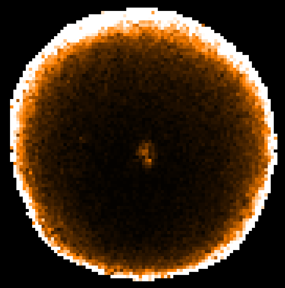
If the MAPVAR=YES option is used when running the SMURF pol2map script, the I, Q and U error estimates in the resulting vector catalogue will be based on the spread of pixel values at each point on the sky in the I, Q and U maps made from individual observations. Thus if 20 observations are processed by pol2map to create a vector catalogue, then each I, Q or U error estimate in the vector catalogue will be based on the spread of 20 independent measurements of I, Q or U. Even though 20 observations is a lot of POL2 data, 20 is still a fairly small number from which to produce an accurate estimate of the error. Consequently, it is usual to see a large level of random “noise” on the error estimates, as in the following example which shows the total intensity (I) error estimates taken from a 12″ vector catalogue near Ophiuchus L 1688 (the noise level increases towards the edge of the map due to there being fewer bolometer samples per pixel near the edge):
The uncertainty on the error estimate can cause some vectors that are clearly wrong (e.g. because they are very different to nearby vectors) to have anomalously low error estimates and so to be included in the set of “good” vectors (i.e. vectors that pass some suitable selection criterion based on the noise estimates).
One simple solution to this could be to apply some spatial smoothing to the error estimates. This would be a reasonable thing to do if there were no compact sources in the map. The errors close to a compact source are generally higher than those in a background region because of things like pointing errors, calibration errors, etc. These things cause a compact source to look slightly different in each observation and so cause higher error estimates in the vector catalogue. The above error estimates map shows this effect in the higher values at the very centre. Simply smoothing this map would spread that central feature out, artificially decreasing the peak error and increasing the errors in the neighbouring background pixels.
An alternative to smoothing is to split the total noise up into several different components, create a model of each component , and then add the models together. The pol2noise script in SMURF has been modified to include a facility to re-model the noise estimates in a vector catalogue using such an approach. This facility is used by setting MODE=REMODEL on the pol2noise command line:
% pol2noise mycat.FIT mode=remodel out=newcat.FIT exptime=iext debiastype=mas
This creates an output catalogue (newcat.FIT) holding a copy of the input catalogue (mycat.FIT), and then calculates new values for all the error columns in the output catalogue. The new I, Q and U error values are first derived from a three component model of the noise in each quantity, and then errors for the derived quantities (PI, P and ANG) are found. New values of PI and P are also found using the specified de-biasing algorithm. The file iext.sdf holds the total intensity coadd map created by pol2map and is used to define the total exposure time in each pixel. The re-modelled total intensity error estimates look like this :
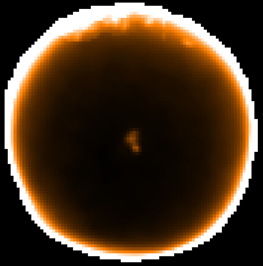
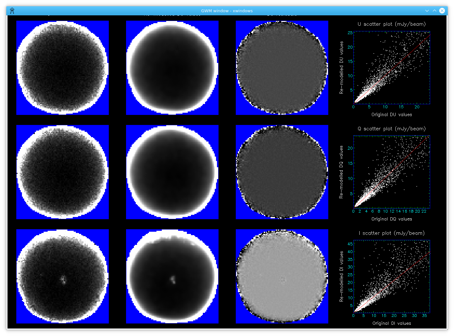
Most of the noise has gone without reducing the resolution. The script displays the original and re-modelled error estimates for each Stokes parameter (I, Q and U), the residuals between the two and a scatter plot. The best fitting straight line through the scatter plot is also displayed:
The three components used to model the error on each Stokes parameter (I, Q or U) are described below:
- The background component: This is derived from an exposure time map (obtained from iext.sdf in the above example). The background component is equal to A.tB , where “t” is the exposure time at each pixel and A and B are constants determined by doing a linear fit between the log of the noise estimate in the catalogue (DQ, DU or DI) and the log of the exposure time (in practice, B is usually close to -0.5). The fit excludes bright source areas, but also excludes a thin rim around the edge of the map where the original noise estimates are subject to large inaccuracies. Since the exposure time map is usually very much smoother than the original noise estimates, the background component is also much smoother.
- The source component: This represents the extra noise found in and around compact sources caused by pointing errors, calibration errors, etc. The background component is first subtracted from the catalogue noise estimates and the residual noise values are then modelled using a collection of Gaussians. This modeling is done using the GaussClumps algorithm provided by the findclumps command in the Starlink CUPID package. The noise residuals are first divided into a number of “islands”, each island being a collection of contiguous pixels with noise residual significantly higher than zero (this is done using the FellWalker algorithm in CUPID). The GaussClumps algorithm is then used to model the noise residuals in each island. The resulting model is smoothed lightly using a Gaussian kernel of FWHM 1.2 pixels.
- The residual component: This represents any noise not accounted for by the other two models. The noise residuals are first found by subtracting the other two components from the original catalogue noise estimates. Any strong outlier values are removed and the results are smoothed more heavily using a Gaussian kernel of FWHM 4 pixels.
The final model is the sum of the above three components. The new DI, DQ and DU values are found independently using the above method. The errors for the derived quantities (DPI, DP and DANG) are then found from DQ, DU and DI using the usual error popagation formulae. Finally new P and PI values are found using a specified form of de-biasing (see parameter DEBIASTYPE).