POL-2 Observing

Current status: Operational

POL-2 is a linear polarimiter (obtaining stokes I, Q and U vectors) installed at the JCMT. The POL-2 is not a detector in istelf and so requires SCUBA-2 and it’s detectors to obtain polarization data.

POL-2 is available at both 850 and 450 microns. POL-2 is used to trace the alignment of dust particles at sub-millimeter wavelengths and thus the magnetic field orientation and strength of regions in our Universe (with some additional physics added into the mix)!

More information about the instrument can be found at the starlink software documentation for POL-2 (sc22).

POL-2 is used in combination with SCUBA-2 and so it has a similar Observing Mode with an 11′ diameter of the final map and scanning at 8″/second during observations.

Noise/time estimates:

An integration time calculator is provided, giving the time to get to an average RMS noise in the 3′ centre of the map – SCUBA-2 ITC in Hedwig.
Larger areas will have to be covered by tiling multiple overlapping daisy observations (see Tiling, below)
Noise levels and sensitivities are briefly discussed below. For a more detailed theoretical discussion of the noise levels in POL-2 maps (and the corresponding total intensity maps derived from them), please see this document.

Our current best prediction for the observing time, t, required to achieve a given RMS, $\sigma$ , at a given transmission, T, is:

$850{\mu}m:\,t_{elapsed}=\frac{1}{f}\left[\left(\frac{763.2}{T_{850}}-64.0\right)\frac{1}{\sigma_{850,mJy}}\right]^{2}$

$450{\mu}m:\,t_{elapsed}=\frac{1}{f}\left[\left(\frac{4626.8}{T_{450}}-411.54\right)\frac{1}{\sigma_{450,mJy}}\right]^{2}$

where f is the sampling factor, defined relative to the default output map pixel size at each wavelength, as:

f₄₅₀ = ( output map pixel size requested / 2 )²and f₈₅₀ = ( output map pixel size requested / 4 )²

These relationships have been incorporated into the SCUBA-2 ITC in Hedwig, the EAO proposal submission system. The POL-2 calculations are available if maptype = POL-2 Daisy is selected in the ITC. For more detail on the sensitivity and the derivation, see section Sensitivity below.

Caveats

The sensitivity analysis was carried out on the blank areas of maps. There will be additional noise factors to consider when observing bright regions.
The sensitivity analysis did not include corrections for the Instrumental Performance (see below).

Contents

1 Noise/time estimates:
- 1.1 Caveats
2 Observing mode:
- 2.1 Instrumental Polarisation Correction
3 Sensitivity
- 3.1 Sources:
4 NEFD as function of transmission
- 4.1 Exposure time as a function of Elapsed Time
- 4.2 Final Sensitivity Equations
5 Tiling

Observing mode:

The observing mode being analysed here is the POL-2 daisy, which is not identical in size/scan speed to the regular SCUBA-2 daisy. Below is an exposure time coverage map for each:

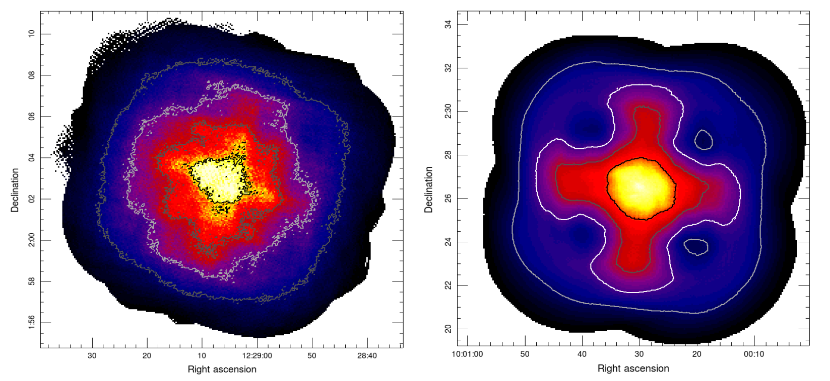
Left: example SCUBA-2 POL-2 exposure time map. Right: “classic” SCUBA-2 CV Daisy . In both images the contours denote the 20, 40, 60 and 80% exposure time levels (compared to the maximum level in the maps). The 20% level extends to ~11′ in diameter in the POL-2 daisy map and ~10.5′ in the CV Daisy map.

During a POL-2 daisy observation, the telescope scans at 8″/s (compared to 155″/s for a CV Daisy scan pattern).

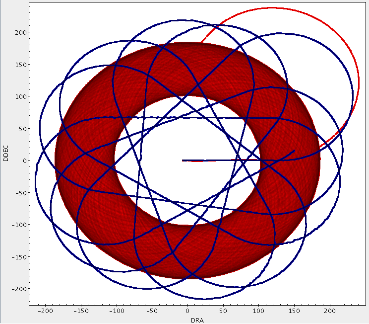
Scan pattern for POL-2 Daisy (blue) vs “classic” SCUBA-2 CV Daisy (red).

Instrumental Polarisation Correction

Instrumental polarisation (IP) can now be performed from a POL-2 dataset alone. It is no longer necessary to have an additional regular (non-polarised) SCUBA-2 map of the source available when reducing the data.

The sensitivity analysis presented below does not include the IP correction.

Sensitivity

The noise sensitivity of the POL-2 maps has been analysed in the same way as was done for SCUBA-2. We looked at observations with point sources at the centre of the map, and:

calculated a noise across the central circle of radius 3′ for each map.
calculated the average ‘exposure time’ per pixel across the central circle of radius 3′ for each map
used this to derive an NEFD (Noise Equivalent Flux Density) to Transmission relation across all the maps.
used the average exposure time to derive an empirical relation between the exposure time in the central map area and the elapsed time of the map.
combined these relationships to get the empirical relationship between the elapsed time of an observation and its RMS, given a specific transmission.

These relationships have been incorporated into the SCUBA-2 ITC in Hedwig. The POL-2 calculations may be accessed by selecting maptype = POL-2 Daisy in the ITC.

Sources:

The sensitivity analysis was conducted using observations of 3C279, 3C273, 3C84 and Uranus. A total of 27 observations were analysed, producing a Q and U map for each observation.

NEFD as function of transmission

The NEFD is calculated as:

$NEFD=\sigma\sqrt{t_{exposure}}$

Where $\sigma$ is the RMS noise for a given map area, and $t_{exposure}$ is the exposure time for that same map area. This NEFD can then be empirically related to the transmission at the time of observation. The figures below show this relation at both wavelengths, using an average NEFD for each map. (Both Q and U maps are shown for each observation).

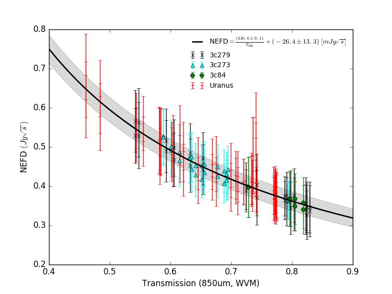
POL-2 850um NEFDs calculated from the noise and exposure time in various maps, and plotted against the transmission at 850um in the map. The noise and exposure time were calculated as averages across the central circle of radius 3′, and excluded a central circle of radius of 30” in order to mask out the point source at the centre of the map. The best fit to the data is shown in the legend.

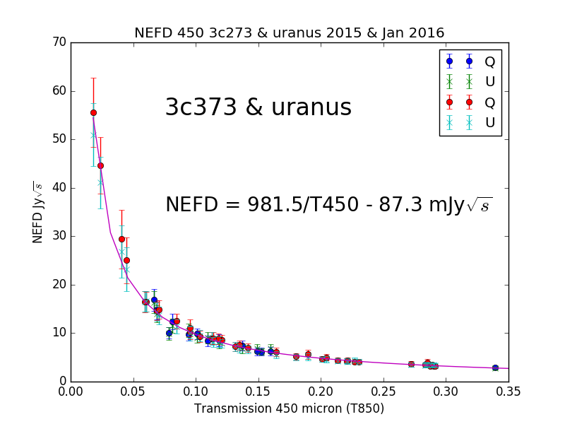
The 450um NEFD plotted vs transmission.
The best fit to the data is shown in the text in the
center of the plot.

The equations relating NEFD to Transmission for each wavelength are then explicitly:

$850{\mu}m:\,NEFD=\frac{310}{T_{850}}-26\,\,\,\,\,\,{\textrm{mJy.}\sqrt{\textrm{s}}$

$450{\mu}m:\,NEFD=\frac{981.5}{T_{450}}-87.3\,\,\,\,\,\,{\textrm{mJy.}\sqrt{\textrm{s}}$

Exposure time as a function of Elapsed Time

A relationship between the average exposure time per 4″ pixel in 3′ radius central circle of our reduced POL-2 850um maps and the elapsed time of the each observation was derived:

$t_{elapsed}=\frac{t_{exp}}{c}=\frac{t_{exp}}{0.165}$

A similar analysis of 450um data produced a c value of 0.045.

Final Sensitivity Equations

Using the definition of NEFD, the empirical relation between NEFD and transmission, and the empirical relation between elapsed time and exposure time, it is possible, for a given transmission, to predict the elapsed time required to yield a desired noise value across the same region of the POL-2 observation and at the same resolution (4″):

$t_{elapsed}=\frac{1}{c}\left(\frac{NEFD}{\sigma}\right)^{2}$

Giving:

$850{\mu}m:\,t_{elapsed}=\frac{1}{0.165}\left[\left(\frac{310}{T_{850}}-26\right)\frac{1}{\sigma_{mJy}}\right]^{2}$
$450{\mu}m:\,t_{elapsed}=\frac{1}{0.045}\left[\left(\frac{981.5}{T_{450}}-87.3\right)\frac{1}{\sigma_{mJy}}\right]^{2}$

Presented in the same format as on http://www.eaobservatory.org/jcmt/instrumentation/continuum/scuba-2/time-and-sensitivity/, these then become:

$850{\mu}m:\,t_{elapsed}=\frac{1}{f}\left[\left(\frac{763.2}{T_{850}}-64.0\right)\frac{1}{\sigma_{850,mJy}}\right]^{2}$

$450{\mu}m:\,t_{elapsed}=\frac{1}{f}\left[\left(\frac{4626.8}{T_{450}}-411.54\right)\frac{1}{\sigma_{450,mJy}}\right]^{2}$

where f is the sampling factor, taking into account the map pixel size relative to the defaults. It is defined as:

f = ( output map pixel size requested / default pixel size )²

At 450 and 850um this becomes:

f₄₅₀ = ( output map pixel size requested / 2 )²and f₈₅₀ = ( output map pixel size requested / 4 )²

These relationships have been incorporated into the SCUBA-2 ITC in Hedwig. The POL-2 calculations are available if maptype = POL-2 Daisy is selected.

Although reliable error estimates have not yet been derived for these predictions, it is possible to see the difference between the actual elapsed time and the predicted time for 850um data using these equations and the figure below.

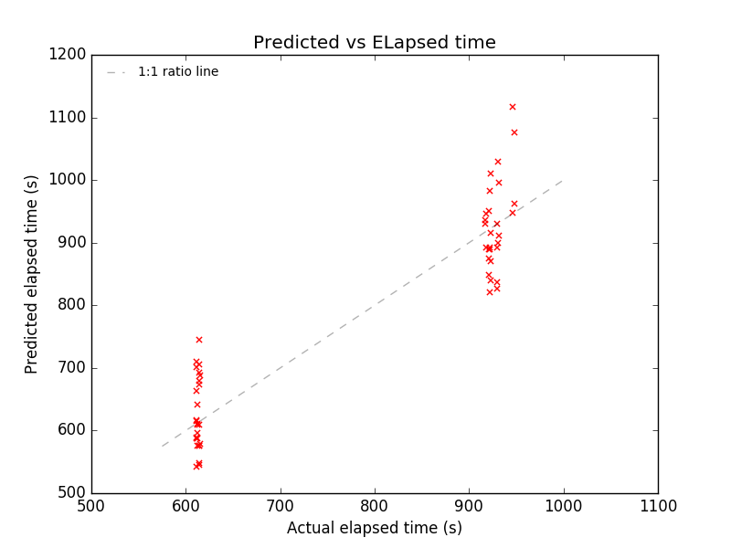
The measured elapsed time from various POL2 850um observations, compared with the predicted elapsed time from the current (2016 February) best sensitivity estimates.

Tiling

The observatory is currently commissioning tiled observations in order to cover areas larger than the central 3′ of an individual scan. Although relatively few details are available so far, potential observers interested in conducting such observations are advised to consider the exposure time pattern of a POL-2 daisy (shown above), as well as the general considerations for SCUBA-2 tiling.