


Contents
Overview
The JCMT offers one “three-cartridge” heterodyne instrument, Nāmakanui (230 GHz and 345 GHz undergoing commissioning, 86 GHz to be commissioned) and one 16-receptor receiver array, HARP (345 GHz).
The Observation Tool (OT) used to define an observation has three modes to map a source using a heterodyne receiver: stare, jiggle or scan mode. Stare mode is used to observe a single point or a set of points one by one by moving the telescope. A jiggle maps the source by moving either the secondary mirror or the telescope. Finally a scan maps the source by continuously scanning the sky. For heterodyne observing the scanning is done by raster scanning the telescope. The mapping method is combined with a switch mode – position, beam or frequency switching – not all switch modes can be combined with all mapping modes.
For large maps the scan (raster) mode is the most efficient observing modes for all receivers – it can only be used with position switching. For a small map a jiggle is most efficient and can be used with position or beam switching. For a single point or a set of single points use a stare observation with beam or position switching. With HARP it is also possible to use frequency switching with the stare and jiggle mapping method.
With beam switching, the secondary mirror is `chopped’ (usually at 1 Hz, and in the azimuth direction, although chopping in any direction is possible) with the source in one beam. At a slower rate, typically every 10-30 seconds, the telescope is moved by an amount equal to the chop throw, to bring the source into the other beam (also called ‘double beam switching’). Thus a negative line signal is obtained when the source is in the reference beam, and a positive one when it is in the signal beam. Both signal and reference phases are necessary; if one attempts to omit the reference part of the cycle, standing waves are the likely result. Generally the technique is effective for sources of small angular size, and should produce better results whenever sky noise is a problem (most of the time). The maximum chop throw is 180 arcseconds. There is a continuum mode for beam switching, where the chop rate is much faster, which can be used if one is interested in the continuum level (e.g. for planets). However this mode is less efficient.
Position switching involves switching between the source and a specified reference position. It can be used with reference positions comparatively far away, but the switching is done rather slowly.
Beam switching produces much better baselines than position switching, which is important for sources with wide lines e.g. extragalactic sources.
Frequency switching involves switching between two target frequencies, rather than two positions on the sky, when observing spectral lines. This can be comparatively fast and efficient under some circumstances, but may not be well suited to certain types of sources (e.g. those exhibiting broad lines or a high density of spectral lines). Frequency switching is not possible with Nāmakanui.
The particulars of how to construct each type of heterodyne observation are given in the OT help pages. There are special considerations to be taken into account when observing sources with a strong continuum such as the moon, the Sun, or planetary atmospheres.
Quick Guide
Source Structure For Jiggles
| Map Size | |
|---|---|
| Compact source | Use a stare |
| Moderate extent (less than 2 arcmins) | Use a jiggle |
| Large extent (greater than 2 arcmins) | Use a scan |
| Little to no emission close (<180″) to target | Use a beam-switched (BMSW) chop to the reference position |
| Contaminating emission near source, or uncertain of region | Use a position-switched (PSSW) observation to a reference further from the source (up to 3 degrees) or frequency switching |
| Primarily after imaging or velocity/frequency data | Select ‘shared offs’ |
| Require accurate flux measurements over extended regions, or spatial smoothing of final map | Select ‘separate offs’ |
| Highly compact core, with well-known position | Select pixel-centered jiggle pattern |
| More extended source, with actual position less known | Select map-centered jiggle pattern |
There are special considerations to be taken into account when observing sources with a strong continuum such as the moon, the Sun, or planetary atmospheres.
Sample observations
Stare (single-sample) or basic grid observations should be used when only a single spectrum (or a few spectral samples), is required on a source position (or several offset positions). If the source is compact, with emission-free positions relatively close (< 180″), beam-switching to a reference position can be used (usually in Azimuth direction, unless one knows that a source is extended in a particular direction). This is called a sample-BMSW, or grid-BMSW. If the region is complex, or has foreground or background emission surrounding it, a position-switch mode, which allows selection of a reference up to three degrees away from the target, can be used instead, and is called a sample-PSSW.
Example with HARP:
HARP has 16 detectors laid out on a 4 × 4 grid, with an on-sky projected beam separation of 30 arcsec. At 345 GHz the beam size is 14 arcsec, and the under-sampled field of view of HARP is 104 × 104 arcsec, as shown in Fig. 4. In a single-pointed observation, the map is under-sampled by a factor of 4.4 in area and by a factor of 17.6 with respect to the Nyquist frequency (λ/2D).
HARP Detector layout (Reference: Buckle et al, MNRAS 2009)
An example of a stare observation, provided from the HARP publication paper, Buckle et al 2009, is shown here. At this time, two receptors were turned off in observations, hence the gaps in two corners.
Grid-position-switch stare observation, with receptors labelled. H00 and H03 have been turned off (top panel). The spectra from each position in the image (bottom panel) (Buckle, et al, MNRAS 2009).
Jiggle-chop and Jiggle-pssw observations
If a source needs to be fully-sampled, and is less than 2 arcmins in extent, the Jiggle-chop or Jiggle-pssw mode is suggested. These observations rapidly step (‘jiggle’) the secondary mirror to observe a grid-pattern of points until the area is fully sampled. A detailed description of the various options for this mode is given below. Again, depending on the surrounding emission in the region, either BMSW or PSSW to a reference position can be selected.
Whilst technically any grid-pattern can be selected for the jiggle mode (e.g. a 3 x 3 or 9 x 9 step map), two pre-designed modes are offered for the HARP array: HARP4, which is a 4 x 4, 16 point jiggle, producing 7.5″ spacing, and is thus slightly under-sampled, and HARP5, a 5 x 5, 25 point jiggle, with 6″ spacing, and slight over-sampling. The spacing for the jiggle mode can also be user-defined for the HARP and Nāmakanui in the JCMT OT.
Example with HARP:
An example for HARP is given here, again from Buckle et al 2009:
Integrated intensity maps of jiggle position-switch observations in 12CO 3 →2 towards a region in Serpens, utilizing the HARP4 pattern (left-hand panel) and HARP5 pattern (right-hand panel). Detectors H00 and H03 have been turned off. Spectra from the same spatial position near the peak are also shown, in a linestyle matching the arrow to the full map (bottom panel) (Buckle, et al 2009).
Scan observations
For regions larger than 2 arcminutes the scan mode is recommended, and is used most often for the array receiver HARP. Regions up to a degree or more in extent can be mapped in a single observation of under an hour when sampling at the fastest rate allowed by the spectrometer back-end, ACSIS. In this ‘raster’ mode, the telescope is moved across a source and the data is integrated and continuously dumped to the back-end (max rate of 100ms). The array is rotated (see image below) to set the sample spacing perpendicular to the scan direction at 7.3 arcsec.
The off position is a single, specified reference position, observed in stare mode, which observes simultaneously an off position for each receptor. The off-source integration time is a factor f greater than the length of the individual scanning sample time so that when combined with the ‘on’ observations, it gives optimum signal-to-noise ratio on the map,  , where N is the number of sample points per row, and t is the sample time. The noise in a single scan does vary due to the change in effective integration time when using an interpolated off-source observation.
A basket-weave technique is normally used with scanning modes in order to minimize the effects of sky and system uncertainties in a map. This technique scans in different directions for each map, so that different receptors are used to sample the same sky point, thus reducing the effects of inaccurate flat-fielding and noisy or non-working receptors. The optimum change is a 90° rotation of the scan direction, which can be set in the OT.
The schematic diagram of a scan observation (Buckle et al 2009)
See here for a comparison of rasters made with HARP using all different available Scan Spacings.
The details:
Jiggle-Chop observations
General description:
This mode of observing is recommended for mapping ≤ 2 arcmin fields where there are emission free positions relatively close (≤ 180″) to the target. Jiggle-Chop (JCHOP) observations utilize (i.e. ‘jiggle’) the secondary mirror to observe a regular grid-pattern of points on the sky as well as sky positions free of emission. To reduce systematics arising from the secondary chopping to one direction on the sky, half the observations are done at a sky position on one side of the target, the other half at a position on the opposite side. This nodding involves moving the whole telescope, but all other offsets require moving only the secondary mirror. This method of observing the sky reference is also referred to as beam-switched.
The advantage of JCHOP observations is that the patterns can be executed quickly, with minimal telescope motions, and that the frequent sky observations result in relatively flat baselines. JCHOP observations are limited to targets that fit within the maximum throw of the secondary mirror of 180″. Both the size of the throw and the direction can be set by the observer in the MSB for the observation, but a customary choice is to chop in AZ i.e. at a constant airmass. If there are no sky positions free of emission within 180″ of the target, the observer will have to select a position-switched observing mode instead.
Jiggle patterns:
The choice of jiggle pattern requires some care and is not straightforward. The detectors of HARP are referred to as receptors and this terminology is used for all heterodyne receivers at the JCMT. The term pixels is used for positions in the output map (of course, all observations will produce a ‘cube’ and the term ‘map’, as used here and below, refers to the spatial area mapped by the observation). A single-receptor receiver, such as Nāmakanui, using a 5×5 jiggle pattern will thus produce a 25-pixel map. HARP, with its 4×4 array of receptors, using a 4×4 pattern will produce a 16×16 = 196 pixel map. Much of the complications associated with the jiggle patterns arise from the centering of the jiggle pattern and where the pointing target will end up in the resulting map:
- A receptor-centered jiggle pattern places the target in the centre of the region mapped by one of the receptors and it will also be on one of the pixels in the output map. All NxN jiggle patterns such as 3×3, 4×4, or 5×5, are receptor-centered and primarily intended for use with the single-receptor receivers or
dual-pol receivers with two receptors on the same position on the sky.
HARP does not have a central receptor. When used with a receptor-centered jiggle pattern it will align one of the inner 4 receptors with the target instead. Hence, when a NxN jiggle pattern is selected with HARP the target will be far off-center in the resulting map, or, stated differently, the map will be very asymmetric around the target position. The orientation of the map is determined by position of the K-mirror, which can be at any of 4 angles, differing by 90 degrees, depending on the elevation of observation. In short, only a region of 1.5×1.5 arcmin will be mapped predictably. Combining observations from different elevations may result in a windmill pattern around that region.
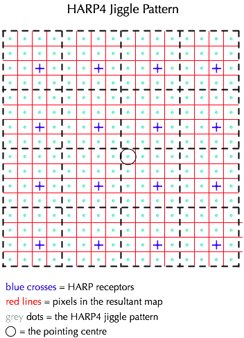
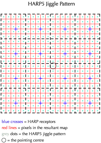
The four special patterns intended for use with HARP that fully sample the footprint of the array are harp4 and harp5, coming in two variations each. The receptors in HARP are spaced 30″ apart and these patterns fill the 30″x30″ postage-stamp of each receptor with ‘4 by 4’ or ‘5 by 5’ points, spaced 7.5″ or 6″ respectively. Compared to a Nyquist sampling of the nominal beam at 345 GHz, the harp4 patterns slightly under-sample, whereas the harp5 patterns over-sample. Harp4 is the recommended pattern for general map making and the cube resulting from the 4×4 receptors of HARP will have 16×16 pixels in e.g. RA, Dec and cover a region of 2×2 arcmins. The harp5 pattern will have 20×20 pixels in RA, Dec covering the same region.
Harp4 and Harp5 can be pixel-centered or map-centered. To understand the distinction one needs to realize that the spatial dimensions of a HARP cube will always have an even number of pixels, i.e. they do not have a central pixel. This presents two choices as to where to position the target in the final map:
- A pixel-centered jiggle pattern will place the target on one of the central 4 pixels of the output map, slightly offset by half a pixel in each direction from the center of the map. As is the case for the receptor-centered map, discussed above, the map will thus be asymmetric around the target but only by
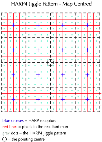
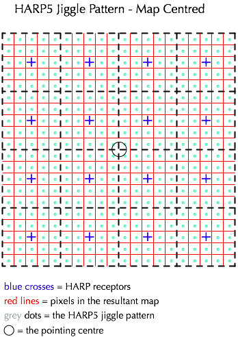
one map pixel. Due to the possible orientations of the K-mirror the edge of the map will this be uncertain by 7.5″ or 6″, respectively. The pixel-centered harp jiggle patterns are named harp4 and harp5 in the JCMTOT. - A map-centered jiggle pattern will place the target exactly in the center of the output map, precisely between the central 4 pixels. The resulting map will be symmetric around the target position and independent of the K-mirror orientation. However, none of the map pixels will align exactly with the target
position, which should not be an issue for an extended source, but might be a concern for a source with a point-like core. The map-centered harp jiggle patterns are named harp4_mc and harp5_mc. Map-centered patterns are also referred to as array-centered since the target is placed on the center of the array between the 4 receptors.
The four harp patterns are illustrated below. The cyan dots in each pattern are the jiggle positions and the centers of the pixels in the output map. In each figure the pointing target is indicated by the small circle and either aligns with a pixel or the center of the map.
An important concept for JCHOP observations is one generally referred to as shared offs (meaning shared sky references). This concept originates from traditional scan-map observations in which the telescope scans across an extended source before pointing to a sky reference. By necessity, all positions observed along the scan will share the same sky reference (off). Since 50% of the noise observed in a spectrum (i.e. on-off) results from the off this would lead to severe ‘striping’ of successive rows unless the integration time in the off position is sufficiently increased so as to drop its noise significantly below the noise of the on measurements. Calculations show that the integration time in the off needs to be multiplied with sqrt(np), where np is the number of on positions in the row. Of course, there is nothing special about scan-maps: the same applies for any observations where a number of points share the sky reference, as is the case for HARP jiggle-maps where the full 4×4 or 5×5 jiggle pattern is observed before going to the off.
Observations benefit from shared offs in two ways, and more so with more points between the offs (the larger the scan-map). To illustrate, consider 1s observations of 16 positions (which would be a very small scan map). Separate offs would require 32s on the sky equally split between ons and offs. Using shared offs, the observation needs only 16+4=20s. But also for each point individually the noise is reduced because of the longer observation of the off. Expressed in a time required to reach a particular rms the combined effect makes shared off observations 4 times faster than separate observations in the limit of many points. More precisely, the factor is ~4/(1+2/sqrt(np)) or ~2.7 for the relatively small HARP jiggle patterns and ignoring fixed overheads (which reduce the factor to closer to ~2). Nevertheless, one night instead of two nights is a huge gain, which is why shared offs are the default for JCHOP observations.
Of course, the above gain comes at a price: all 16 or 25 jiggle-positions from every receptor are correlated because they have the same sky reference (off). As long as the pixels are kept separate this is not an issue because noise remains dominated by the on measurement and the points can be regarded to be only weakly correlated. However, any operation in which pixels are combined will ‘suffer’ from this correlation in the sense that it will combine pixels that are not fully independent and the noise will hence not drop with the customary sqrt(np) factor. Note that this both applies to operations that use a spatial convolution (smoothing) as well as total flux measurements that sum or average over pixels such as aperture photometry. In the extreme, when averaging data over the whole footprint of a harp4 observation, the noise will be 1/4th (16 independent receptors) instead of 1/16th (196 pixels) of the noise per pixel. Finally: note that JCHOP continuum mode observations always will have separate offs because there will be only a single jiggle position per sky reference.
In conclusion: if imaging or velocity/frequency data are the primary aim of the observations, shared offs are hugely beneficial and recommended; if accurate flux measurements over extended regions are the primary aim or the final maps will be spatially smoothed significantly, separate offs are recommended instead.
More details can be found here.
Jiggle-Position Switch observations
General description:
(Since Jiggle-position switch observations share many characteristics with the Jiggle-chops, please make sure to have read the previous section).
This mode is recommended for mapping ≤ 2 arcmin fields where an emission free position is relatively far away from the target. Jiggle-PSSW (JPSSW) observations utilize the secondary to observe a regular grid-pattern of points but, contrary to JCHOP, use a position-switch of the whole telescope to observe sky positions free of emission.
The advantage of JPSSW over JCHOP is that sky reference positions are not restricted to a distance within 180″ from the target and can be as far as degrees away. The main disadvantages are the less accurate sky subtraction due to the larger switch and the longer time between sky references. Another disadvantage is the additional overhead resulting from moving the whole telescope to the reference position. The position can be specified as either a relative position or a fixed position. The switch will be to this single position only rather than two positions on diametrically opposite sides of the target, as is the case for JCHOP. (However, note that the reference position can be defined in a coordinate system other than RA, Dec resulting in it rotating from observation to observation in that frame). In order to minimize the number of moves, the telescope executes an OFF-ONs-ONs-OFF etc. pattern, with the switches pairs-wise associated.
Jiggle patterns:
More details can be found here.
Grid Position-Switch
General description:
This mode of observing is recommended for sparse mapping or irregular patterns. Grid-PSSW (GPSSW) observations don’t use motions of the secondary mirror, but instead move the telescope between the target grid-positions as well as sky positions free of emission. Likewise, it is possible to do Grid-BMSW observations, but these will not be further discussed here.
The advantage of Grid-PSSW observations is that the target positions are under full control of the observer and that under-sampled maps or non-regular patterns can be observed. Like JPSSW, the sky reference can be far away from the target. A disadvantage is that moving the telescope to execute the grid is relatively slow resulting in a larger overhead than with jiggle observations. In order to minimize the number of moves, the telescope executes an OFF-ONs-ONs-OFF etc. pattern, with the switches pairs-wise associated. The off-switch will be to a single, specified, reference position. (However, note that the reference position can be defined in a coordinate system other than RA, Dec resulting in it rotating from observation to observation in that frame).
[Note: it is possible to do a grid of jiggle-maps by putting a “Jiggle-Eye” inside an “Offset” iterator. However, in this case the jiggles will be executed as fully independent observations at each grid point, resulting in independent cubes.]
Grid patterns:
Grid patterns can be set up using the Offset iterator in the JCMTOT, either as a regular pattern or as a list of individual offsets.
Shared and separate modes are available as for JCHOP (see description there), but without being able to do a fast jiggle to cover the pattern the distinction is rather irrelevant in practice. With a minimum of 1s/point and a maximum of 30s between refs, multiple grid-points can only be observed for short integration times. This means that relatively many telescope moves are required for little integration time implying large overheads. Being more efficient, shared offs mitigate the effects of the increased overheads. On the other hand, short observations with separate offs are particularly inefficient: because of restrictions imposed by the data handling within the correlator these observations have to switch to the reference after each grid-point, even if the integration time per point is only as short as 1s.
Finally, as soon as the integration time per grid-point becomes such that only a single grid-point can be observed before having to go the sky reference (i.e. 15sec by default) there will be only one point per reference and the distinction between separate and shared offs disappears: the observations will use separate offs.
In conclusion: for any observations with integration times ≥15s per grid-point the choice of shared or separate offs is irrelevant. For shorter integration times a choice for separate offs comes with a heavy penalty in the form of excessive overheads.
More details can be found here.
Frequency-Switch observations
Frequency-switch mode observing is possible for HARP observations. However it is an involved process that requires additional support and effort from the observer. Observers need to consider telluric lines (CO, Ozone that changes with time) and know that the baselines are in general sinusoidal. Reductions of such data are not currently handled well by ORAC_DR.
General description:
Frequency switching mode is suitable for sources with narrow lines (~< 10 MHz) and low line density. In such sources it has superior noise performance for single point observations or small maps. Frequency switching also has advantages in large maps when there is no nearby line free region to use as a reference position.
Baselines:
Non-flat Baselines are common with frequency switching. There are several reasons for this. The frequency change and the associated variation in LO power changes the mixer impedance, coupling and conversion efficiency creating baselines. For small frequency switches the baselines are well behaved and can be removed by baselining. Another cause is standing waves in the optics in front of the mixer. These will move in the band pass when the frequency shifts and are not cancelled. The standing wave between the cabin and secondary has a frequency of ~ 16.2 MHz at the JCMT. Frequency switching by 16.2 or 32.4 MHz reduces such standing waves. Thus frequency switching is most suitable for observations of narrow lines not affected by baselines. It should definitely not be used for continuum observations. The JCMT uses an elaborate calibration scheme to reduce the baselines which doubles the time integrating on calibration loads.
Frequency switch amount:
The baselines and the performance of the LO system limits the amount of the frequency shift. Currently switches up to 32.4 MHz have been tested with good results for both RxA and HARP. Since the line is present in both the signal and reference observation it will occur twice in the raw spectrum. After processing to average the two independent lines in the spectra there will be three features. This is not a problem for an isolated line but care has to be taken if there is more than one line in the band pass. Users should also be aware that lines from the earth’s atmosphere not are canceled. Terrestrial Ozone lines are routinely observed using frequency switching. Thus CO and Ozone can generate additional features in the spectra. The user needs to select center frequency (or velocity) and switch amount to avoid line blends.
Noise performance and map size:
Due to the fact the same line is observed both in the source and reference spectra the noise is improved by sqrt(2) after processing. However, observing modes that uses one reference observations (offs) for several on sources positions as jiggles and grids (with shared offs) and scan pssw becomes more efficient when the number of on source positions are large. Neglecting overheads these methods are more efficient than frequency switching if more than 5 on source points share the same off. The actual trade of point depends on overheads. Thus, in cases where there not is a good reference position in the vicinity of the source, frequency switch can maintain the advantages for larger maps. However, it is still recommended that the calibration is performed on a line free reference position. This requires that a reference position is defined in the OT target component. In cases with weak lines (line << Tsys) and no continuum it is possible to calibrate on source.
A discussion Observing Using Frequency Switching can be found in the Spring 2010 JCMT Newsletter.
Issues from Large Position Switches
Large Position switches are best avoided, as they can cause baseline ripples. In essence there are two types of ripples seen in the baseline of spectra. A a slow ripple that is typically caused by differences in reflection looking at the cold load. This creates uneven calibration within is easily seen when having a DC offset. For instance created by a large position switch in elevation.
Additionally in some of the spectra a fast ripple typically for reflection between the mixer and sub-reflector is seen – although not neccessarily caused by large position switches.