


Overview
Observations of strong continuum sources such as bright planets as well as the Moon and Sun need special considerations. Two effects increase the noise. First the Tsys on the source is significantly higher than off source due to the continuum from the source itself. The Heterodyne Integration Time Calculator (ITC) does not take this into account, making the time estimate too optimistic. Secondly the noise in the calibration observation contributes to the noise level, which the ITC does not consider at all. The second issue can be severe, limiting the effective observing time in an observation to about the time spent on the calibration rather than the time spent on the source. The standard calibration time is 5 seconds. The exact level of degradation depends on the ratio between the continuum level and Tsys.
The first issue requires the observing time on source to be extended, the second issue requires the calibration time to be extended. It should be noted that these considerations also affect the peak of very bright lines e.g. the CO line from Orion Molecular Cloud 1 complex (OMC 1). The noise level on the peak is higher than on the baseline. It is the latter the ITC estimates. Currently there is no software in the ITC or the JCMT observing tool (JCMTOT) to estimate the degradation or automatically adjust the on source or calibration times. Such adjustments would be source strength and Tsys dependent.
Increased Calibration Times
To observe a target with a heterodyne instrument, the telescope points to the field that is “ON-source” (ON) and to a field that is “OFF-source” (OFF) for the same amount of time. The OFF data is then subtracted from the ON data to eliminate any background noise contributing to the source. When the calibration observations are executed, an ambient temperature absorber (sometimes called the “hot load”) is periodically placed into the beam at a point between the receiver and the secondary mirror to allow for the determination of TA*: the antenna temperature corrected for atmospheric absorption and ambient temperature telescope losses, including hot spillover and blockage (see Penzias & Burrus, 1973, for details). Then, the OFF position (and a “COLD load” in the case of HARP observations) is observed.
The default time spent on the Ambient load, OFF position (during the calibration cycle), and COLD load (when using HARP) is 5 seconds each. For low-level continuum sources, this generates a noise level in the calibration data (Ambient – OFF) that is a small percentage of the overall noise budget. When calibrating observations of strong continuum sources, however, the integration time spent on the Ambient and OFF positions must be increased to ensure the noise level of the calibration data (Ambient-OFF) is as low as in the (ON-OFF) data, since the (ON-OFF) difference in continuum level will be significant. Without increasing the integration time of the calibration observations, the calibration noise will dominate, making the observations extremely inefficient.
For strong continuum sources, the Ambient and OFF loads observed during the calibration cycle need to be observed for at least the same amount of time as the regular ON/OFF observations. There is no way, however, to increase the calibration integration time in the JCMTOT. This must be performed by the telescope operator “on-the-fly” while observations are being carried out. In the MSBs, an “observer note” should be included with specific details about how long to increase the calibration integration time and labelled “IMPORTANT CALIBRATION INFORMATION”; in this way, the TSS will take the appropriate action.
Overheads
When planning the necessary time required for your strong-continuum program, the ITC will not accurately calculate the overall time required to achieve your target RMS and the MSBs in the JCMTOT will not accurately display the amount of time required to execute the observations. This is due to the increased overheads of extending the time spent observing calibration targets. For Nāmakanui observations, the calibration cycle consists of an Ambient load and the OFF position. For HARP observations, the calibration cycle consists of an Ambient load, a COLD load, and the OFF position.
Example
A strong-continuum observation that integrates for 2 minutes ON SOURCE will require:
- 2 minutes on COLD LOAD (HARP OBSERVATIONS ONLY) — Calibration
- 2 minutes on OFF position — Calibration
- 2 minutes on Ambient load — Calibration
- 2 minutes on SOURCE — Target
- 2 minutes on OFF — For background subtraction
= 8 minutes Total for Nāmakanui
= 10 minutes Total for HARP(+time for slewing, etc.)
With the default 5 second calibrations (which is what the ITC and JCMTOT will assume), this same observation would only take just over 4 minutes to execute. **Calibration is performed at the start of each observation and after ~30 minutes if the MSB is long.**
To increase the efficiency of the observations, the most ideal situation is to reduce or eliminate the continuum difference between the ON and OFF positions. One solution is “Frequency Switching” (where the instrument is tuned to a different frequency rather than pointed at a physical “OFF” position) but this observation method often has issues with baseline rippling and it is currently unsupported for Nāmakanui. If the continuum source is wide enough and the science program is analysing differences between one side of the source and another (for instance comparing physical conditions across the atmosphere of Venus), one can also target the source so the ON and OFF positions are both “on” the target but at different locations, yielding a comparable continuum level in both the ON and OFF fields.
Flat Fielding Uncertainties: 16.5 MHz Baseline Ripple
Ideally, the bandpass gain should be the same while targeting the COLD, Ambient, ON, and OFF positions. Optical reflections that generate standing waves, however, are slightly different when observing the Ambient load and the Sky (since the Ambient load is a physically introduced component in the optical path). The reflections occur between the secondary mirror and the receiver and between the dewar windows or filters and the receiver. These reflections introduce imperfections in the flat fielding which manifests as a variation in the continuum level for strong continuum sources. Empirically, observing a strong continuum source like Venus results in a ripple in the baseline with a period of approximately 16.5 MHz at the level of a few % to 5%. The phase of the ripple will vary with elevation.
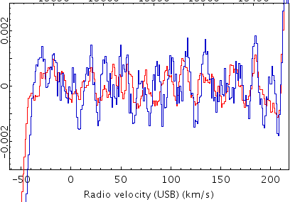
Figure 1: Blue = 1 subscan of a strong continuum source. Red = 40 subscans, co-added. The baseline ripple must be removed before the RMS will decrease as the square root of the integration time. This is especially important for sensitive observations of faint lines.
Other Considerations
For strong continuum observations performed close to the Sun (or pointed directly at the Sun), temperature gradients across the primary dish generated by the heat of the Sun will result in beam degradation and, subsequently, higher calibration uncertainties. Daytime observations can only be carried out until ~3pm Hawaiʻi standard time (01:00 UTC) to allow for dish recovery before the start of evening observations.