

Contents
Scan Patterns
There are two observing modes available with SCUBA-2; CV Daisy for point sources and a rotating Pong pattern for larger scale mapping. The choice of rotating Pong pattern will rely on two dependent factors: (i) the size of the region you wish to observe (ii) the size scales of extended structures you wish to recover.
CV Daisy
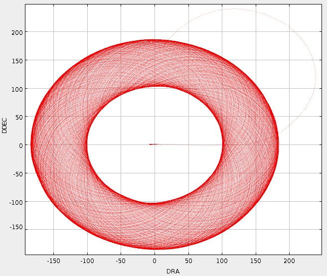
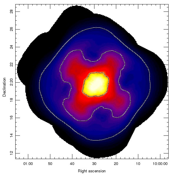
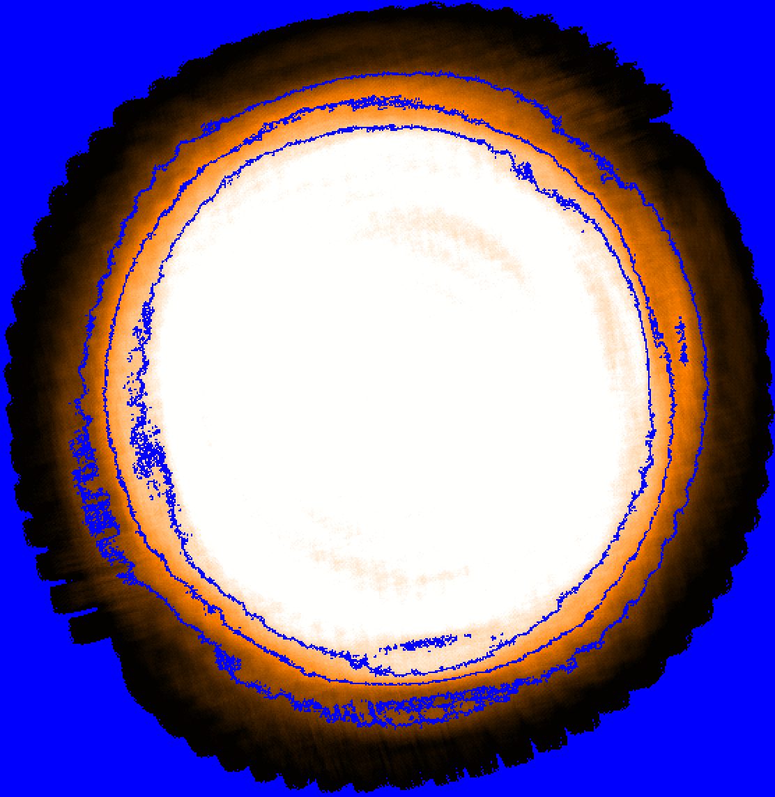
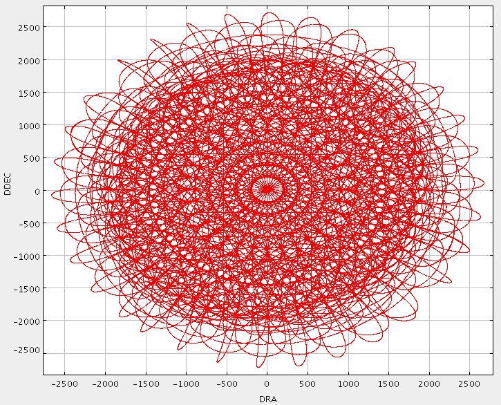
A “CV Daisy” (CV = constant velocity) is designed for small and compact sources of order 3-arcmin or less, although there is significant exposure time in the map out to 12-arcmin. The telescope executes a pseudo-circular pattern at a speed of 155″/s. This pattern keeps the target coordinate on the array throughout the integration.
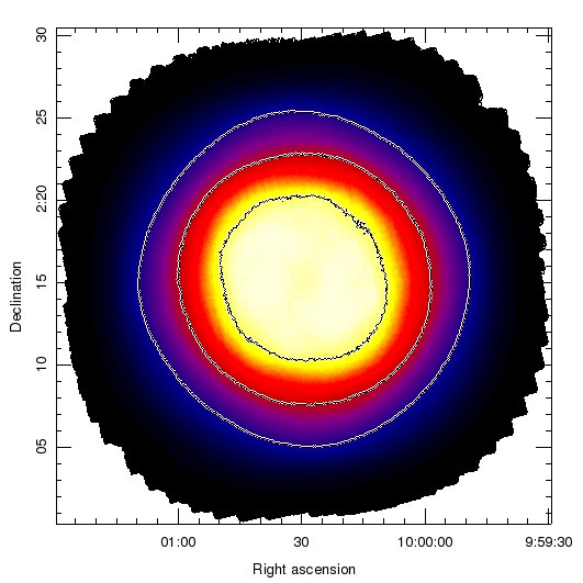
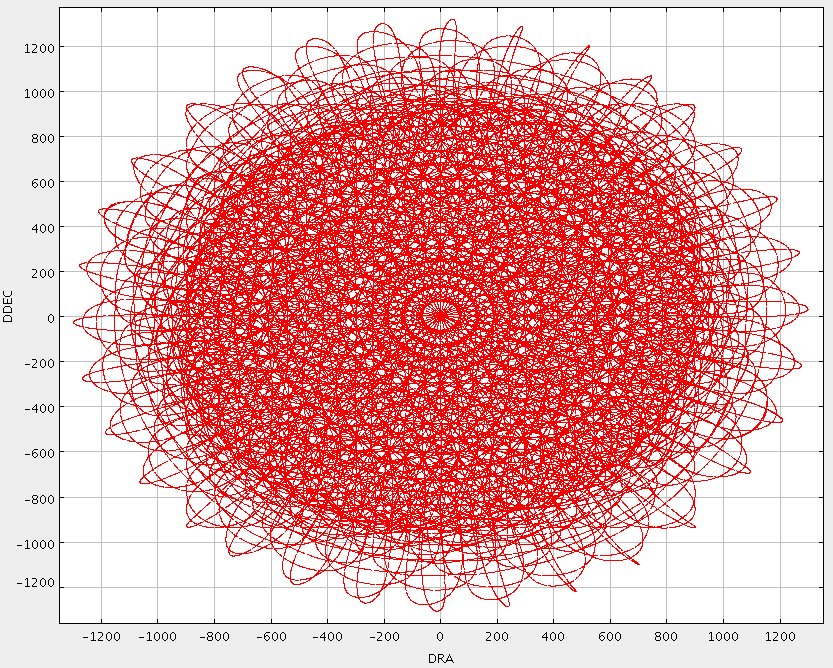
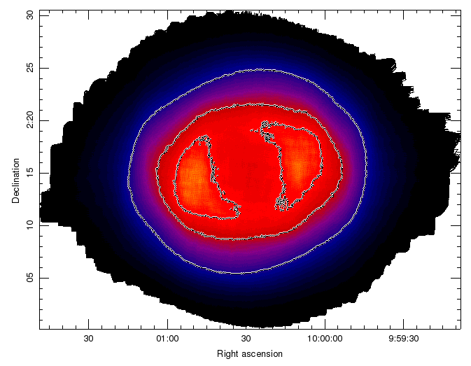
The telescope track for this pattern is shown in the graph on the right below. The exposure time map for a typical observation is shown in the image on the right below. The image is scaled between 0-600 seconds. Contours indicating 100, 250 and 500 seconds are shown.
Rotating Pong patterns
These are designed for mapping larger fields, and there are five sizes currently available (defined by their diameter): 900″, 1800″, 2700″, 3600″ and 7200″. The telescope tracks across the defined sky area, filling it in by “bouncing” off the walls of this area. Once a pattern is complete the map is rotated and the pattern repeated at the new angle.
A full rotating Pong pattern with all repeats is set to take 40 minutes. Decreasing the number of repeats decreases the overall exposure time. The parameter space of the telescope velocity, the spacing between successive rows of the basic pattern and the number of rotations have been explored to determine those which give the most uniform coverage across the requested field.
15-arcmin Pong map
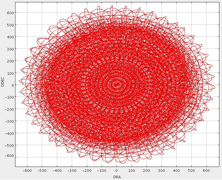
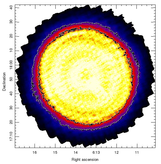
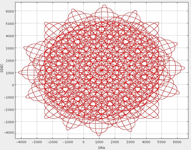
The 15-arcmin Pong map (also known as pong900) pattern has a scan spacing of 30″, telescope velocity of 280″/s with 11 rotations of the field (~ 8deg apart) within a ~40 minute integration.
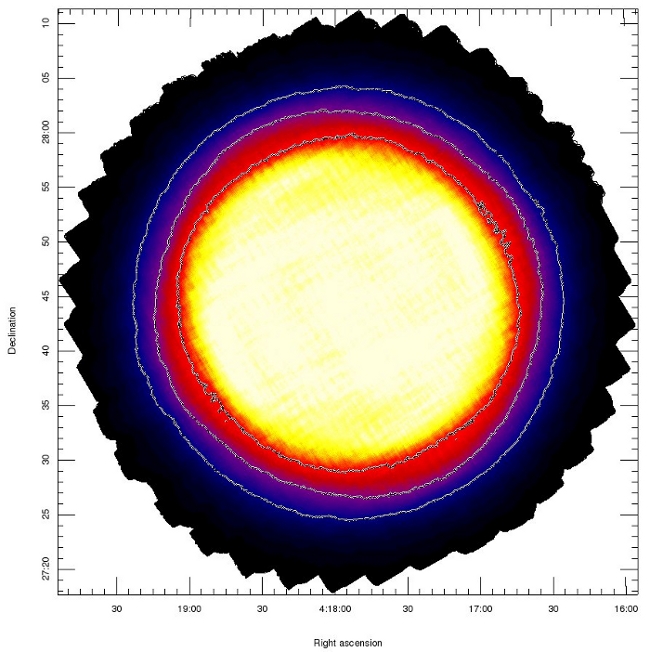
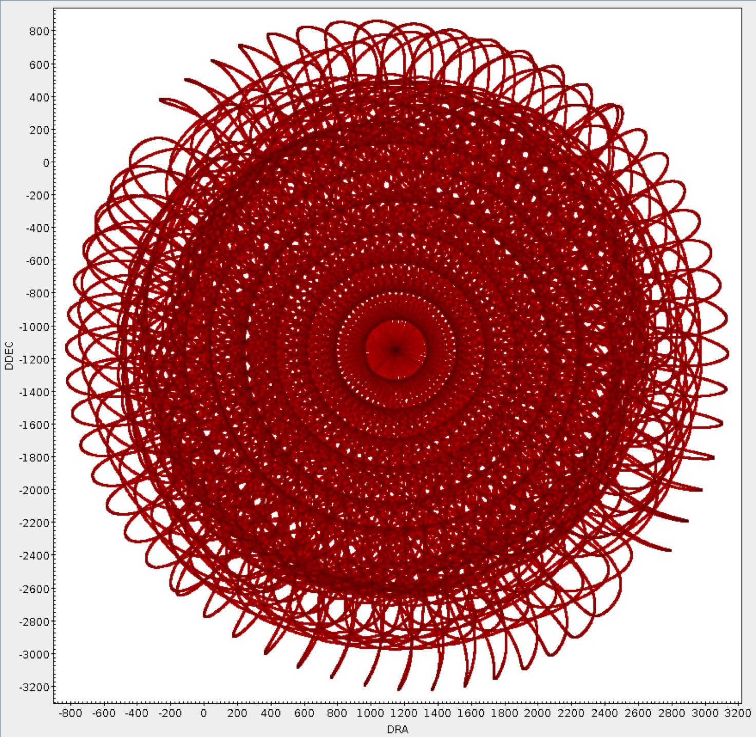
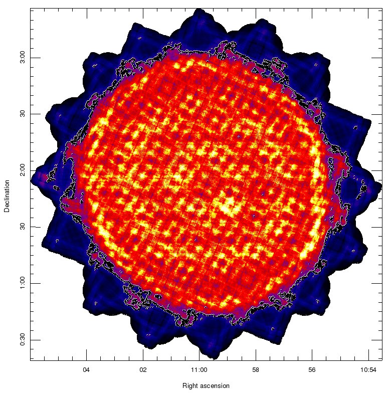
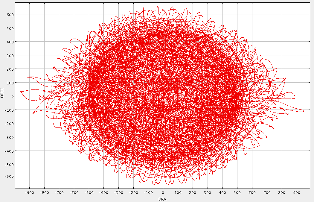
The telescope track for this pattern is shown in the graph below. The exposure time map for a typical observation is shown in the other image below. The image is scaled between 0-160 seconds. Contours indicating 50, 100 and 150 seconds are shown.
30-arcmin Pong map
The 30-arcmin Pong map (also known as pong1800) pattern has a scan spacing of 60″, telescope velocity of 400″/s with 8 rotations of the field (~ 11.25 deg apart) within a ~40 minute integration.
The telescope track for this pattern is shown in the graph below. The exposure time map for a typical observation is shown in the other image. The image is scaled between 0-40 seconds. Contours indicating 10, 20 and 30 seconds are shown.
45-arcmin Pong map
The 45-arcmin Pong map (also known as pong2700) pattern has a scan spacing of 105″, a telescope velocity of 540″/s with 8 rotations of the field within a ~40 minute integration.
The telescope track for this pattern is shown in the graph below. The exposure time map for a typical observation is shown in the other image. The latter image is scaled between 0.5-11 seconds. Contours indicating 3, 6 and 9 seconds are shown.
1-degree Pong map
The 1-degree Pong map (also known as pong3600) pattern has a scan spacing of 180″, telescope velocity of 600″/s with 8 rotations of the field (~ 11deg apart) within a ~40 minute integration.
The telescope track for this pattern is shown in the graph below. The exposure time map for a typical observation is shown in the other image. The image is scaled between 0-9 seconds. Contours indicating the 3.5 and 7 seconds are shown.
2-degree Pong map
The 2-degree Pong map (also known as pong7200) pattern has a scan spacing of 360″, telescope velocity of 600″/s with 4 rotations of the field (~ 23deg apart) within a ~40 minute integration.
The telescope track for this pattern is shown in the graph below. The exposure time map for a typical observation is shown in the other image. The image is scaled between 0-3 seconds. Contours indicating the 1.2 seconds are shown.
A Daisy or a 15-arcmin Pong?
An issue that appears to come up regularly is that a pong900 is used when possibly a CV Daisy would have been better, given that the latter is much faster and actually gives significant exposure time out to 12
arcmins. The numbers break down as follows:
For the same integration time, the rms in the center of a Daisy will be more than twice as good as in a pong900. Out to a radius of about 5.5 arcmin the noise will still be below the pong900 target noise. Beyond this radius the noise will exceed the target noise, but that is also the case for the pong900 (see the radial profiles below).
I.e. the trade-off is between a flatter and slightly larger map (pong900) and a somewhat smaller but much deeper map in the center with a distinct noise gradient across the field (CV Daisy).
Detection experiments may well be better off with Daisies, although statistical conclusions, such as number counts, may become more complicated. The same may be true for isolated (i.e. non-mosaicked) fields where one could ask if the negative impact of the noise gradient and a smaller field out-weigh the benefits of a deeper mapping across most of the image.
There are other possibilities, such as doing an initial exploratory Daisy to the required depth in a 3-arcmin field (this can be done in less that 25% of the time it takes for a pong900) and then proceed with pongs on the most promising candidate(s). Pong and Daisy fields can be combined. It may also be beneficial to use a pattern of offset Daisies to mitigate somewhat for the more pronounced gradient or to better match the source morphology in the field.
High elevation constraints
By monitoring observations taken over a range of dates an elevation dependence in the exposure time has been found for all maps. This elevation dependence appears to affect 15′ pong maps observed at elevations greater than 65 degrees. The plot below shows the median exposure time the inner 1.5′ radius of the map.
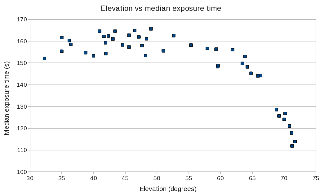
An example of the telescope track and exposure map is given below. This particular observation was taken over an elevation range of 69-73degrees. The image on the left is scaled between 0-160 seconds. Contours indicating 50, 100 and 120 seconds are shown.
Because of this we adopt an elevation restriction of 70 degrees for all pong maps and of 75 degrees for CV daisies.
NEFD versus transmission
The NEP corresponds to the noise in the raw data and is a combination of intrument and atmospheric noise. Measured NEPs in pW are shown on the plots below:
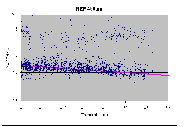
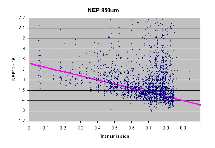
It should be noted that these measurements were taken from the first 10 seconds of data from a large number of observations without much selection on data quality. A number of effects can be seen. In the 450μm data there is a secondary track at NEP ~4.75e-16. These are times that an array (mostly s4c) for unknown reasons ‘locks’ into a noisier state. The same effect is present in the 850μm data (mostly the s8d array), but is much less apparent.
The magenta line shows the adopted fits to the data, which follow the lower edge of the distribution but are displaced to the median distribution of the NEP. However, at 850μm the NEP can be significantly worse than that on occasion! The cause of this is unclear at present and under active investigation, but appears to be atmospheric or environmental in nature and not intrinsic to the instrument. Please make sure to revisit this page prior to the submission deadline for the latest information on this issue.
By applying a nominal FCFs (537 @ 850μm and 491 @ 450μm) and a correction for the atmospheric attenuation at the respective wavelengths (see Integration times page) the NEP can be converted to a NEFD. These, along with the above fits, are shown in the next plots as a function of transmission, T. Note that these are for a single, average bolometer and not the focal plane as a whole.
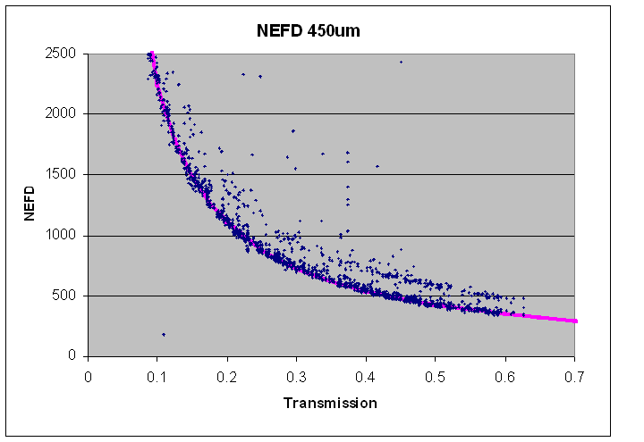
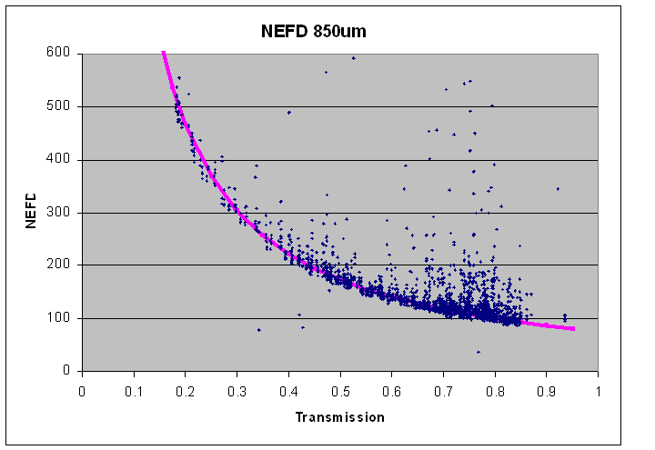
The linear fits of the NEP data then translate to the following equations for the effective NEFD, i.e. representative for the focal plane as a whole by adding the 1/sqrt factor:
\frac{1}{\sqrt_{3670}}}mJy\sqrt{s})
\frac{1}{\sqrt_{3630}}}mJy\sqrt{s})
These equations, together with the exposure versus elapse relations from the next section, form the basis for the integration time relations.
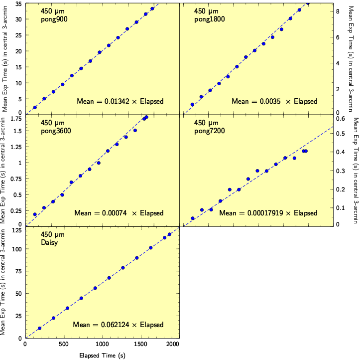
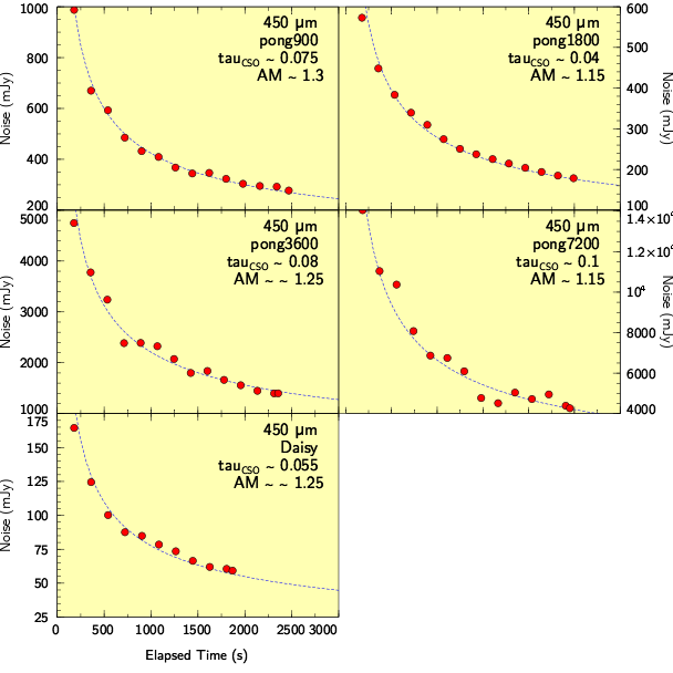
Noise integration
The graphs below show how the exposure time in the central 3-arcmin of the map increases with the elapsed time of the integration, and also how the noise per pixel in that same region decreases. Note that in all cases the noise integrates down with the square-root of time, as expected. Furthermore, although these relations can give an indication of how long it will take to get to a certain depth, it is only applicable for the conditions reported (air-mass, AM, and CSO tau). We advise that you use the relations on the main SCUBA-2 integration time calculation page.


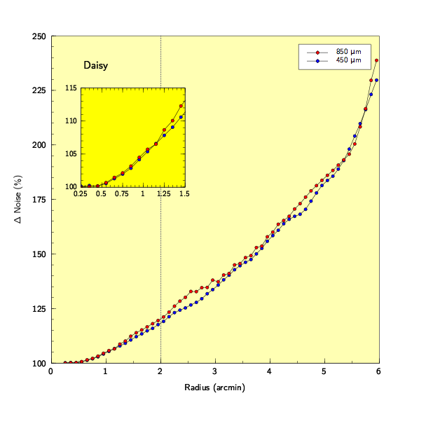
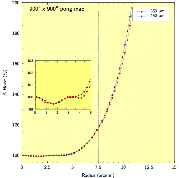
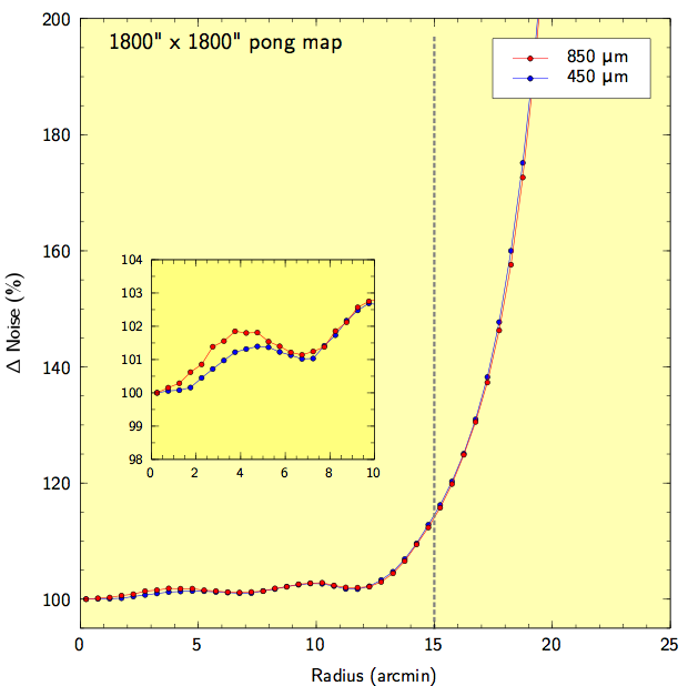
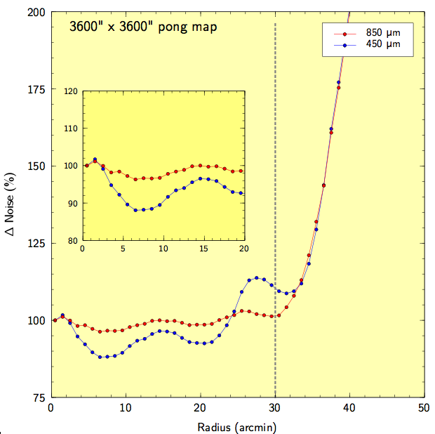
Radial dependence of noise in maps
For each of the standard map sizes, the (square root of the) exposure time in the map is used as a proxy for noise, and this is calculated as a function of radius. The graphs below show the uniformity of that noise across each map, with the grey dashed line signifying the demanded image size.
Below, the noise profile for the CV daisy observing mode is shown. This mapping mode is designed for point sources. Nevertheless, given the noise increases by ~35% out to a radius of 3-arcmin, this mode is still useful for mapping intermediate-sized, or compact, fields of the order of 3-6 arcmin.
The graphs below show the same but for 15-arcmin, 30-arcmin, 1 degree and 2 degree pong maps. The noise remains quite uniform across the field, never getting above a 20% difference, relative to the centre of the map, by the edge of the demanded field size.
Filtering SCUBA-2 data and large scale structure
In contrast to SCUBA-2’s predecessor, SCUBA which observed an area of sky while simultaneously chopping, SCUBA-2 removes atmospheric noise in the data processing stage. The power spectrum of data taken by SCUBA-2 has a 1/f noise curve at lower frequencies. To ensure source signals are far away from this 1/f region of the power spectrum, fast scan speeds are required. The maximum size of the structure that can be recovered from the power spectrum is determined by the scan speed and frequency cut applied to the data:
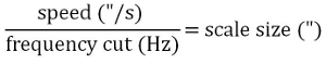
When chosing your map size from the options above you should consider the scanning speed for that size pong. If you wish to recover large scale extended structure you are advised to use large pongs that scan at a faster rate rather than tiling smaller pong maps. Ultimately it is the size of the SCUBA-2 FOV that determines the sensitivity to large scale structure. Below is an image of the SCUBA-2 footprint with the eight sub arrays labeled.
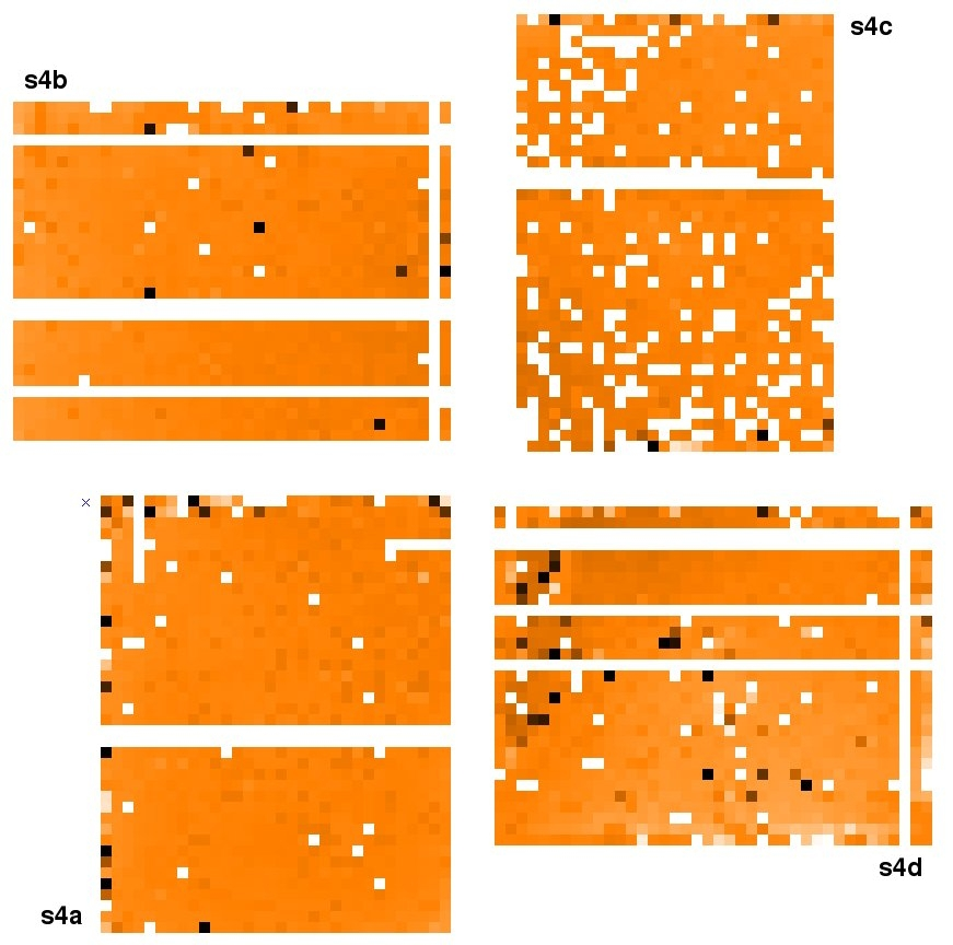
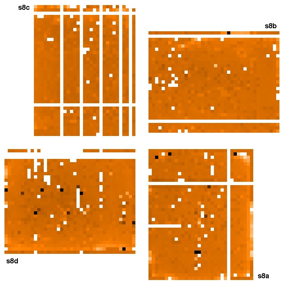
Typically SCUBA-2 is referred to as having a field of view (FOV) of 8 square arc minutes. As you see in the image above the FOV is not quite square and as such a FOV a value of approximately 600” is more representative. Removal of correlated signal typically sky or instrumental noise, which is common to all bolometers reduces the ability to detect contiguous structures larger than the FOV. This is referred to as common mode subtraction.
On a final note, during data reduction common mode subtraction on a per array basis is discouraged for sources not considered to be compact.