


POL-2 is the JCMT’s sub-millimeter polarimeter working at both 450 and 850 microns. POL-2 is a polarimeter not a detector, and so requires SCUBA-2 for use. It is used to trace the alignment of dust particles at sub-millimeter wavelengths and thus the magnetic field orientation and strength (with some additional physics added into the mix) of regions in our Universe!
Recently it has been found that sometime there is a loss of synchronisation between data values and pointing information in the data reduction process (CALCQU, run by pol2map as part of step 1). This loss of synchronisation is triggered by anomalous values in the array of HWP (Half Wave Plate) angles stored in the raw data. The result is blurring (or smoothing) of sources in some POL-2 maps (see figure below).
The fix is to download our rsync this build of the starlink software and re-reduce your data. If you look at your re-reduce data you may find that some of your maps improve, depending on whether any of your observations suffered from the blurring problem. The size of the improvement will depend on how many blurred observations you have.
For regions where multiple observations were used to produce the final maps the issue may have been less pronounced if obsweight=yes was used.
In addition, users wishing to reduce POL-2 450 micron data are asked to ensure the data have been reduced using the latest starlink 2018A software prior to this release there was a bug in the software which caused a 4 degree difference in the angular zero point at 850 and 450, so all 450 vector maps produced so far will have a systematic error of 4 degrees in the vector angle, unless updated software (rsync starlink or 2018A starlink) was used.
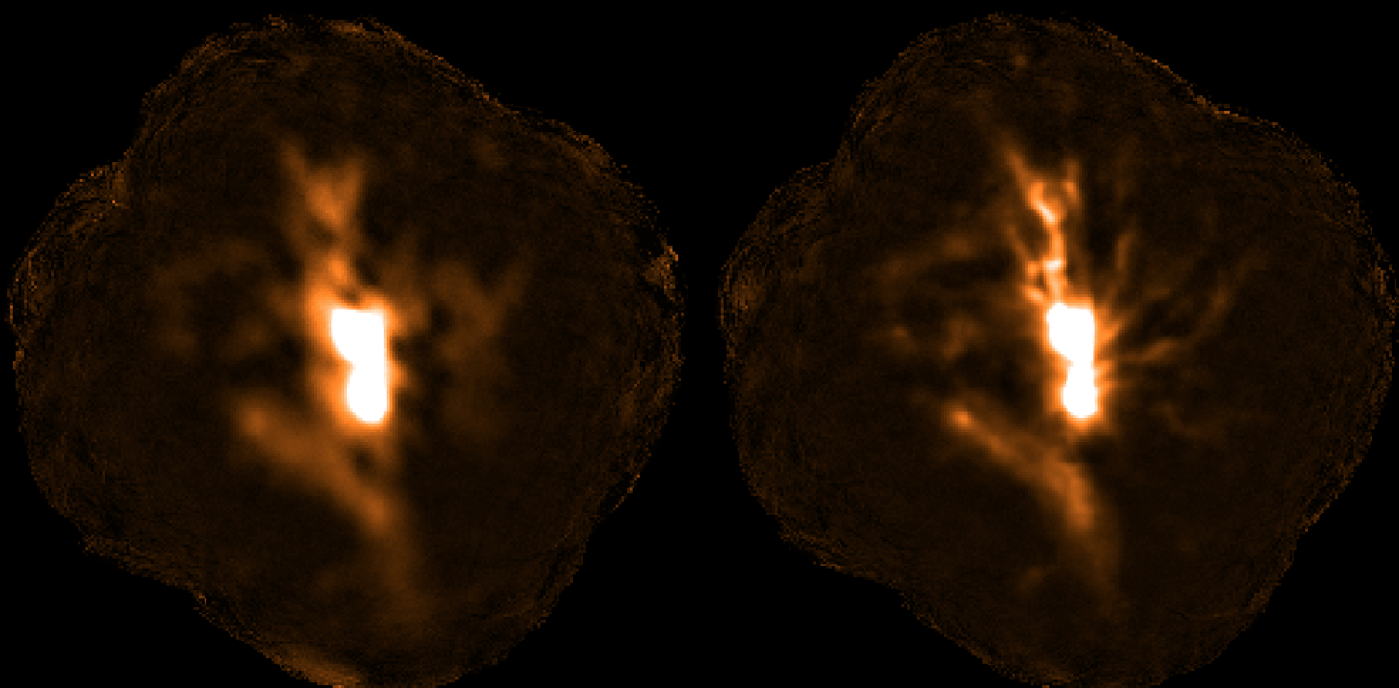
The image shows two total intensity maps made from an observation of OMC1. Left: before the fix for blurring. Right: after the fix for blurring.
Also did you know you can combine various I maps into a cube to view as a movie? You can do this (assuming you ran pol2map with “mapdir=maps”) by running:
kappa
paste in=maps/\*Imap out=Icube shift=\[0,0,1\]
gaia Icube
Then in gaia, in the pop-up window that holds the cube visualisation controls, drag the “Index of plane” slider left or right to step through the planes in the cube!
You can do the same for the Q or U maps by replacing “I” with “Q” or “U” above (note, that’s an upper case “I” for the externally masked I maps – use a lower case “i” for the auto-masked I maps).
– 20180724