


Note: This tutorial assumes that the computer to be used already has a functioning installation of a recent version of the Starlink software suite (the latest release is available for download here).
Basic Pipeline Reduction
This tutorial demonstrates how to run a standard, basic reduction of a heterodyne observation using the ORAC-DR pipeline software and provides an introduction to basic Gaia use.
The ORAC-DR pipeline is a generic automated data reduction pipeline that can process your raw JCMT data and return advanced data products: baselined single observation cubes, mosaicked and co-added cubes, moments map and clump catalogues. Before you begin we recommend reading Chapter 5 of the The Heterodyne Data Reduction Cookbook which discusses the ACSIS Pipeline.
- Obtain a copy of the file JCMT_HETERODYNE_tutorial_2016.tar.gz containing the raw data. Copy this file to a suitable directory to work in (~/data is used in the following example):
cp JCMT_HETERODYNE_tutorial_2016.tar.gz ~/data - Switch to the data directory and open the tarball:
tar xvzf JCMT_HETERODYNE_tutorial_2016.tar.gzThis directory should now contain a number of .sdf files corresponding to different heterodyne observing modes which are to be reduced by different recipes:
Observation (UT Date + Scan Number) Source Observed Spectral Line Mode Type of Data 20110103 Scan 25 L1551-IRS5 C18O(3-2) Stare Narrow Line 20160317 Scan 17 CRL 618 CO(3-2) Stare Broad Line 20110926 Scan 29 CRL 2688 CO(3-2) Stare (wide band mode) Gradient 20160316 Scan 39 Mars CO(3-2) Stare Continuum 20111025 Scan 7 G34.3+0.2 CH3OH(7-6) Stare Line forest 20070705 Scan 34 G34.3+0.2 CO(3-2) HARP-5 Jiggle map Gradient 20070705 Scans 38+39 G34.3+0.2 CO(3-2) Raster map (basket-weave) Gradient - before proceeding further you will need to ensure the starlink software is loaded in your terminal, and you have loaded the analysis tools package; Kappa.Firstly, in case there is uncertainty as to which shell is currently in use, type the following to find out the answer:
echo "$SHELL"If using the Bash or zsh shells, type:
export STARLINK_DIR=/starOr, if using the TC-shell or C-shell, instead type:
- It is possible to inspect a raw data file with Gaia:
gaia a20110103_00025_01_0001.sdf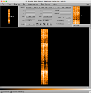
One of the heterodyne tutorial datasets imaged in Gaia.
- Before reducing your data it is possible to look at the metadata using fitslist and ndftrace (for more information about the metadata click here):
fitslist a20110103_00025_01_0001.sdfand:
ndftrace a20110103_00025_01_0001.sdf - It is possible to check the System Temperature (Tsys) and Receiver Temperature (Trx) by doing an hdstrace on your data:
hdstrace a20110103_00025_01_0001.MORE.ACSIS.TSYSand:
hdstrace a20110103_00025_01_0001.MORE.ACSIS.TRX
- Set up ORAC-DR for ACSIS data processing, and specify that the reduced files will be written to the current working directory:
oracdr_acsisBy default, ORAC-DR will issue a warning that the default input data directory does not exist. It is therefore necessary to manually set the ORAC_DATA_IN environment variable.
If in the Bash or zsh shells, type:
export ORAC_DATA_IN=.Or, if in the TC-shell or C-shell, type:
setenv ORAC_DATA_IN . - Next, create a file mylist with the absolute file path to the raw data. This can be done via:
ls /absolute/file/path/file-of-interest.sdf > mylistInitially it is recommended to only reduce a single file at a time (typically one source/frequency set-up)
- It should now be possible to run ORAC-DR by typing the following:
oracdr -files mylist
ORAC-DR will use the default recipe specified in the header (REDUCE_SCIENCE) to reduce the data. This should launch a separate windows showing the progress of the data reduction. It will also indicate any problems encountered, and report as files are created and/or deleted. The -nodisplay option is not necessary. Although often informative, displaying the outputs from the reduction process while running it may slow down its execution.
Once the reduction process has completed, press the Exit ORAC-DR button to close the window. A number of files should have been produced as a result of the reduction process, including various logs, NDF and PNG preview image files. REDUCE_SCIENCE uses REDUCE_STANDARD for standard calibration sources and REDUCE_SCIENCE_GRADIENT for maps. Note that REDUCE_STANDARD does not produce group files. Alternatively (for to see progress in the terminal, and a log saved to the directory you are working in) try:
oracdr -files mylist -nodisplay -log sfA list of the output files produced and their descriptions can be found here:
- It is possible to examine the reduced group dataset in Gaia. This can be done by typing:
gaia a20110103_00025_01_reduced001.sdf &or
gaia ga20110103_25_1_reduced001.sdf &This should launch a main Gaia window with the reduced image in it. It is possible to zoom in and out of the image using the two Z buttons. Click on a pixel to view the spectrum at this position. It is then possible to click on the Send: replace button to view the spectrum in SPLAT.
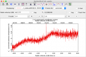
A spectrum from the heterodyne tutorial dataset displayed in SPLAT.
Gaia and SPLAT have many other features to aid in image analysis. Feel free to experiment!
- Estimation of the rms of a spectrum can be done in SPLAT using the Σ button (“Get statistics on region of spectrum”), by “adding” new background regions and calculating the statistics. Alternatively you can simply run the kappa stats command on the error component of the data:
stats file.sdf comp=error
setenv STARLINK_DIR /star
Then in any of the above shells, type:
source $STARLINK_DIR/etc/profile
And then launch Kappa by typing:
kappa
If you encouter issues, please ensure you have installed Starlink correctly. You can also consult the Starlink support mailing list for questions/concerns (or email helpdesk@eaobservatory.org).


Other JCMT data reduction/analysis tutorials are available here.