


Note: This tutorial assumes a pre-existing installation of the latest version of the Starlink software suite (available here), and that it has been initialized. The steps outlined below are for the BASH and ZSH shells; if the TCSH or CSH shell is being used, please replace the export command with the appropriate setenv equivalent. See Step 4 of SCUBA-2 DR Tutorial 1 for an example of how to do this. Please also remember to run KAPPA and SMURF first.
Matched Filters
Matched filters are a method of wavelet analysis used for optimal detection of point sources, by removing the large scale structure for a map and convolving the remaining information with an image of the telescope beam. Some ORAC-DR recipes (e.g. REDUCE_SCAN_FAINT_POINT_SOURCES) will automatically carry out matched filtering on the group coadds produced by the pipeline. This tutorial will demonstrate how to use PICARD to perform the same filtering on an already-reduced map.
The map used for this is a single observation with one visible faint point source present. Better examples of matched filtering can show a map going from appearing blank to having obviously detected point sources. When using matched filtering, care is needed in interpreting the flux of the output sources. See 6.1 of Starlink document SUN/264, and section 8.7 and Appendix D of SC/21 (The SCUBA-2 Data Reduction Cookbook) for more details on the SCUBA-2 Matched Filter.
- Download the example data from here and copy it into a working directory on your computer:
JCMTTutorial-MatchFilter.tar.gz - Gunzip and untar this file:
tar xvfz JCMTTutorial-MatchFilter.tar.gzYou will now have a JCMTTutorial-MatchFilter directory, containing a reduced SCUBA-2 observation in NDF format, and a README file.
- Examine the files:
cd JCMTTutorial-MatchFilter

ls

README.txt jcmts20140729_00011_850_reduced001_obs_000.sdf
This observation is a reduced SCUBA-2 Pong map taken by the JCMT Cosmology Legacy Survey on 2014-07-29. The date and scan number may be deduced from the file name, and the file metadata can be examined with the KAPPA command fitslist:
fitslist jcmts20140729_00011_850_reduced001_obs_000.sdf - Run the standard matched filter on it. Starlink provides a PICARD recipe for doing this, which can be run like so:
export ORAC_DATA_OUT=. (setenv ORAC_DATA_OUT ./ if you are using TC shell)

picard -log sf SCUBA2_MATCHED_FILTER jcmts20140729_00011_850_reduced001_obs_000.sdf
Read the messages written to screen, which are also saved in a log file that begins with .picard.
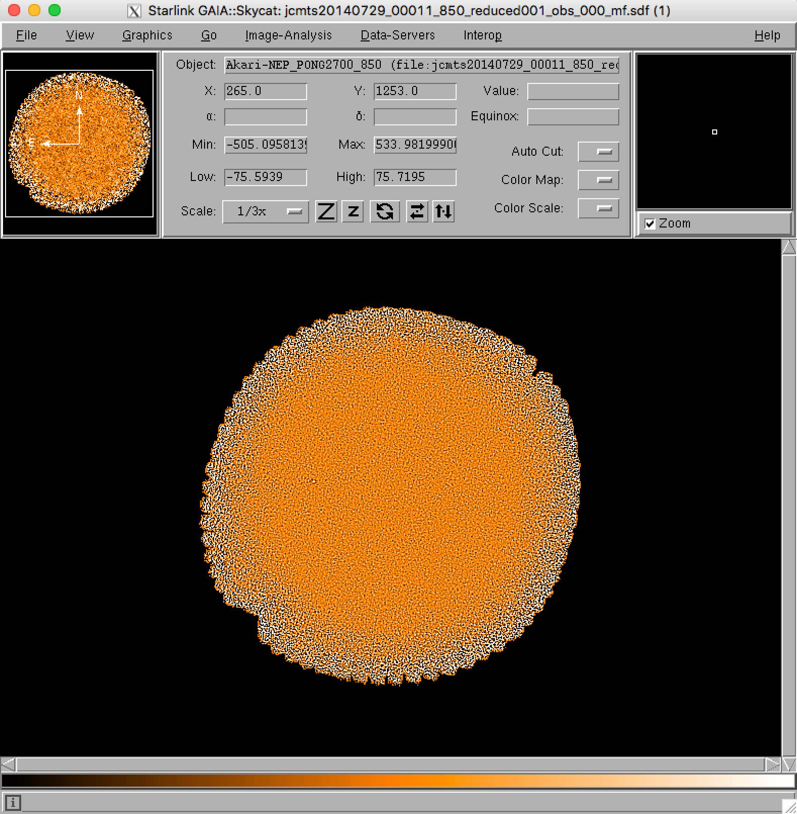
- Open the matched filter image (extension _mf) in Gaia, and compare with the original image. Various source finding and photometry methods can be used to compare the before and after cases. GAIA enables the user to interactively perform photometry on a displayed file.
- Look at the background structure of the matched filter image. There is a characteristic pattern visible in it, which is recognizable in comparison with a normal SCUBA-2 map. Note that when searching for data in the JCMT Science archive, it may be possible for the user to recognize which observations were reduced with a matched filter just from this pattern visible in the preview image.
Picard-generated map of SCUBA-2 Tutorial 4 dataset using matched filtering.
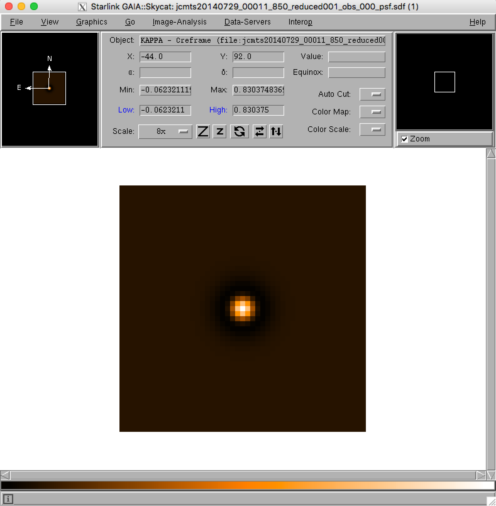
- The point spread function (PSF) used by the recipe is stored in the file with the _psf extension.

The standard Point Spread Function (PSF) used in SCUBA-2 Tutorial 4 (zoomed).
Advanced Tips
This can be run on a standard JCMT calibrator source to see the effect on the beam – try downloading a reduced observation of (e.g.) Arp 220 from the JCMT Science Archive here and running this PICARD recipe on it. Look at the difference in the source before and after running matched filtering. it is also possible to manually use the KAPPA beamfit command to analyze the maps.
The SCUBA2_MATCHED_FILTER PICARD recipe takes various optional recipe parameters. It is possible to set the following recpars to change the defaults:
- Change the point spread function (by default it will construct one based on the measured SCUBA-2 beam from Dempsey et al. 2013):
PSF_MATCHFILTERName of an NDF file containing a suitable PSF. Must exist in the current working directory. If not specified, the recipe will calculate one itself for each input file.
- Change the normalization scheme used for the PSF:
PSF_NORMNormalization scheme used for the PSF created by this recipe if one is not specified using the above parameter. This may be PEAK or SUM to indicate whether the Gaussian PSF should have a peak of unity or a sum of unity. If not specified, the recipe assumes PEAK.
- Whether to SMOOTH the data (default is 1, indicating it should be smoothed):
SMOOTH_DATAFlag to denote whether or not the image and PSF should be smoothed and have the smoothed version subtracted from the original. If not specified, the recipe assumes a value of 1 (smooth and subtract).
- The FWHM of the Gaussian used to smooth the data:
SMOOTH_FWHMFWHM of Gaussian used to smooth data and PSF images before convolving with the PSF. If not specified the recipe assumes a value of 30 arcsec.
Other JCMT data reduction/analysis tutorials are available here.