


Note: This tutorial assumes that the computer to be used already has a functioning installation of a recent (2017A or newer) version of the Starlink software suite (the latest release is available for download here). The user is also advised to first obtain basic familiarity with SCUBA-2 datasets, via the relevant JCMT web pages and associated (non-POL-2) SCUBA-2 data reduction tutorials. Steps 4 and 5 of this tutorial together currently take ~45 minutes to run on a 2015 Apple MacBook Pro computer with a quad-core 2.2 GHz Intel Core i7 and 16GB of RAM, and a full reduction may therefore be impractical to run during a live tutorial session. Two data file options are therefore offered, one containing the raw data, and one including the reduced data reduction products.
Additional Note: Users should bear in mind that POL-2 is a new instrument and that both commissioning and software development are an ongoing effort.
Basic Reduction of a Single Observation Using the SMURF pol2map Command
This tutorial demonstrates how to run a basic, standard reduction of a SCUBA-2 POL-2 dataset using the Starlink software suite. The SMURF command pol2map can be used to considerably simplify this process. This command will perform all the necessary reduction steps, and although the results produced may improve with subsequent Starlink releases, the command invocation is not expected to change significantly. In the longer term, the usual oracdr command will support routine POL-2 data reduction. For further background and details on the material covered in this tutorial, please consult the POL-2 Cookbook (Starlink document SC/22), which is distributed as part of the public Starlink software distribution.
Before proceeding further you should ensure the Starlink software is loaded in your terminal, and you have loaded the analysis tools package; smurf:
starlink
smurf
if you have issues please ensure you have installed starlink correctly, you can also see the Starlink support mailing list for questions/concerns (or email helpdesk@eaobservatory.org).
Note that in the following tutorial, it is possible, but not necessary, to include the .sdf filename suffix when specifying a Starlink data file as input or output.
- OBTAINING THE TUTORIAL DATA AND SETTING UP THE DIRECTORIES: Obtain a copy of the file JCMT_POL-2_tutorial1_2017_raw_only.tar.gz (file size: ~1.9 GB) containing the tutorial raw data. This is the only file needed if the user plans to run through the whole tutorial at his/her leisure. A second file is also available, however, containing the data reduction products generated during the tutorial, and is primarily recommended for use when available time is limited (e.g. during live tutorials). This is available at JCMT_POL-2_tutorial1_2019_reduced_only.tar.gz (file size: ~279 MB), and should be placed and unzipped in the exact same directory location as the first tar file. If the reduced data tarball is also used, then steps 4 and 5 below (the data reduction steps) can be skipped. These files contain POL-2 850-micron band observational data for the well-known quasar 3C 273.
- COPY OVER THE TARBALL: Copy the relevant file(s) to a suitable directory to work in (e.g. your local home directory, ~/ , in the following example):
cp JCMT_POL-2_tutorial1_2017*.tar.gz ~/ - UNPACK THE TARBALL: Switch to the working directory, open the tarball and change to the newly-created directory containing the raw data:
cd ~/

tar xvzf JCMT_POL-2_tutorial1_2017*.tar.gz

cd tutorial/raw
This directory should contain a number of .sdf files and a README document. This can be checked by listing the contents of the directory by typing:
lsThe dataset used in this example is made up of just one observation. Observation 43 is a POL-2 4.4′ × 4.4′ POLCV_DAISY of duration 931s.
- CREATE A FILE CONTAINING THE LIST OF THE INPUT DATA FILENAMES AND USE IT TO GENERATE AN INITIAL UNPOLARIZED TOTAL INTENSITY MAP: As of Starlink version 2017A, it is no longer necessary to also have a non-polarimetric Instrumental Polarization (IP) reference map of the total intensity: the new SMURF pol2map command generates the required information directly from the polarimetric dataset. This also means that future POL-2 proposals no longer need to request a dedicated accompanying unpolarized SCUBA-2 observation for IP correction purposes. It is first usual to create a text file (here called mylist) listing all of the input files (including their explicit pathnames), move it into the reduced data directory, and then use that directory as the current working directory (pol2map will be run from there later on). This can be done via the following commands:
ls -d -1 $PWD/*043*.sdf > mylistIt is then useful to create a directory for the temporary files produced under the pol2map.Do this using:
mv mylist ../reduced/
cd ../reduced/mkdir tmpThen, use (for tcsh/sh shells):
setenv STAR_TEMP tmp/or (for Bash/zsh shells):
export STAR_TEMP=tmp/The pol2map command may then be run on the raw polarization data (observation 43) with the following command to generate an initial I map:
pol2map in=^mylist iout=iauto qout=! uout=! mapdir=maps qudir=qudataThe mylist file created previously is used to specify the list of files that will be used for input. The iout parameter is set to specify that an unpolarized total intensity map file called iauto.sdf will be produced, using an automatically-generated astronomical mask. Note that qout and uout are set to null values in the above, as no Q or U maps are to be produced during this initial reduction stage. Finally, local target directories called maps/ and qudata/ are specified as the locations into which the resultant maps and Q and U data respectively for each separate observation are to be written.
- PRODUCE THE FINAL I, Q AND U MAPS, AND THE VECTOR CATALOGUE: Now that an initial I map is available for use in IP correction, the last stages of the polarimetry reduction can be run together via a single command. The following invocation of pol2map will generate the final intensity and polarimetric maps, and an associated vector catalogue:
pol2map in=qudata/\* iout=iext qout=qext uout=uext mapdir=maps mask=iauto maskout1=astmask maskout2=pcamask ipref=iext cat=20160125_00043_cat debias=yes binsize=12The parameters specified in the above command are as follows:
- in: The input Q, U and I time-stream data files to be used. These were created by the first run of pol2map described above.
- iout: The resultant final total intensity map, named iext.sdf in this example.
- qout: The resultant combined final Q map; named qext.sdf in this example.
- uout: The resultant combined final U map; named uext.sdf in this example.
- mapdir:The directory containing the individual I, Q and U maps from each separate observation _Imap.sdf, _Qmap.sdf and _Umap.sdf.
- mask: The preexisting mask to be used as input during the reduction, named iauto.sdf in this example. This was created in step 4 (above).
- maskout1: The first (AST) output mask generated by this pol2map run and used in the creation of the final I, Q and U maps; named astmask.sdf in this example.
- maskout2: The second (PCA) output mask generated by this pol2map run and used in the creation of the final I, Q and U maps; named pcamask.sdf in this example.
- ipref:The non-polarimetric reference map to be used for IP correction; named iext in this example. The specified file (“iext.sdf”) is the same one specified for parameter “iout” – the script first creates it as an output and then uses it as an input.
- cat: The output FITS file generated containing the polarization vector catalogue; named 20160125_00043_cat.FIT in this example.
- debias: This parameter is set to TRUE here to specify that a correction for statistical bias is to be made to the percentage polarization and polarized intensity values in the output vector catalogue (see above).
- binsize: Set this parameter to the bin size you wish to use for your output vector catalogue. Changing this value is a good first check of reliability.
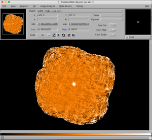
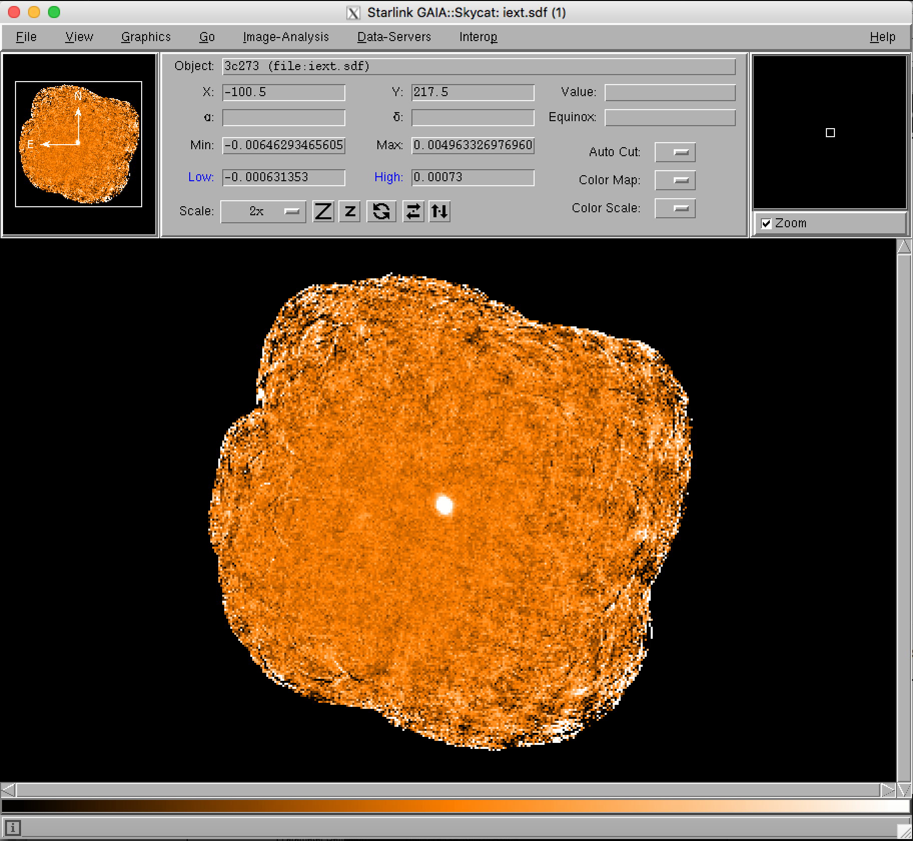
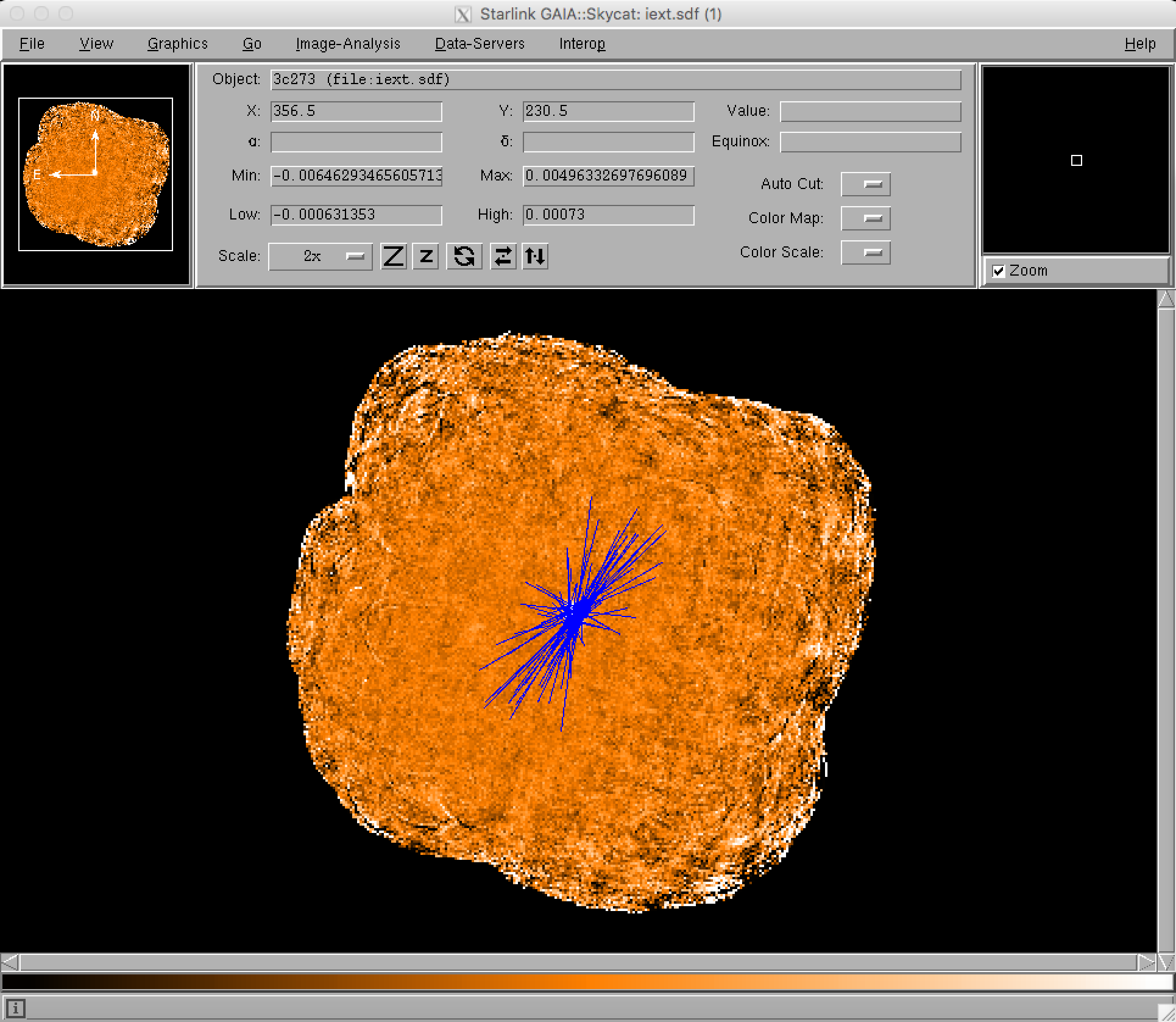
- DISPLAYING THE MAPS: The Starlink data visualization tool Gaia can be used to inspect the results of the data reduction. To do this, we will first image the total intensity map, and then overlay the polarization vectors. The following command may be used to image the total intensity map:
gaia iext.sdf &Note that it may be helpful to adjust the scale of the image using the Scale option in the main Gaia window:
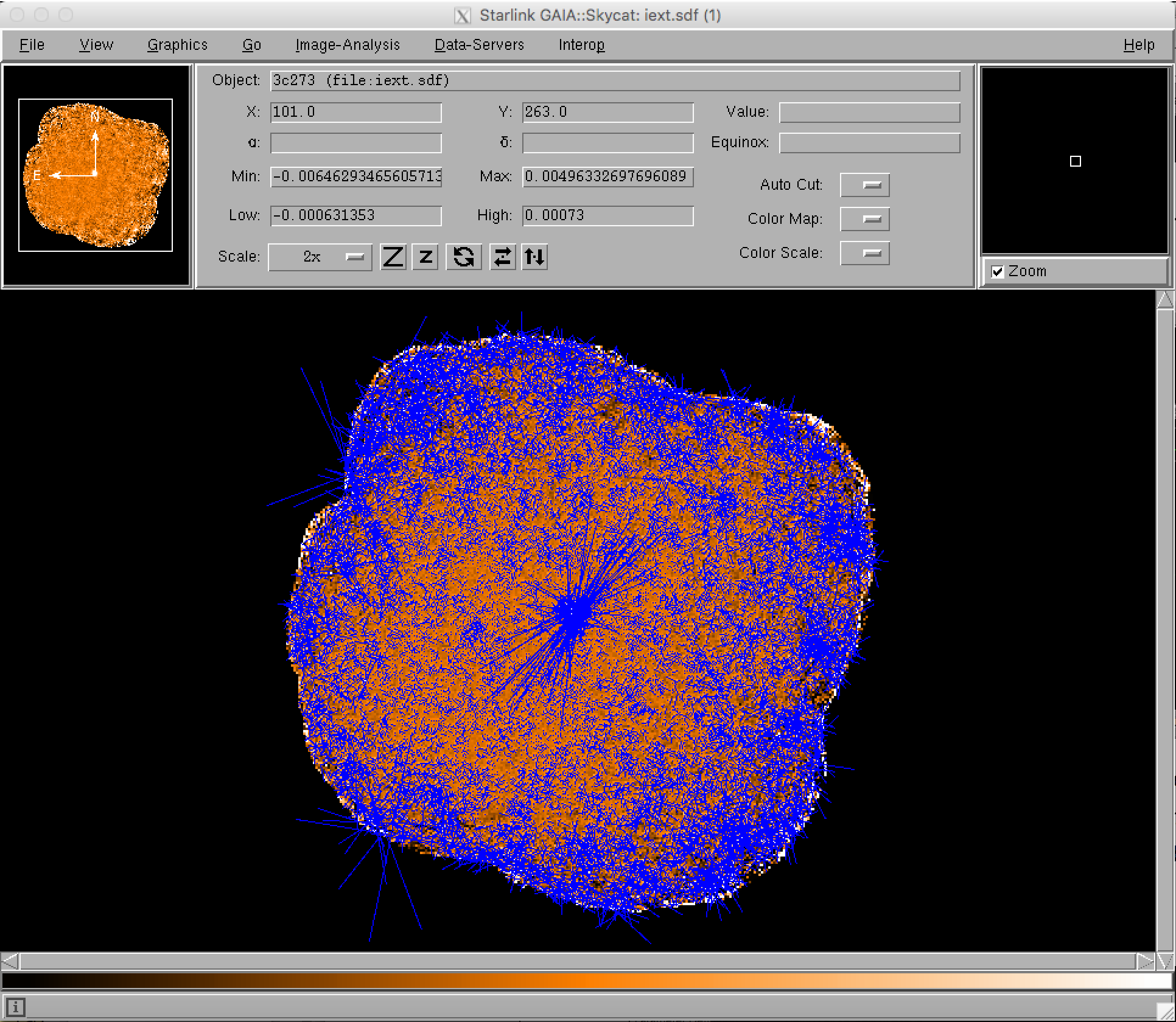
 Next, in the main Gaia window, select the drop-down menu option Image-Analysis / Polarimetry toolbox…. This should launch a new toolbox window entitled GAIA: Polarimetry. From this window, use the drop-down menu option File / Open to load the file 20160125_00043_cat.FIT. This should then populate the lower part of the window with the contents of this polarimetry catalogue file, and a very large number of vectors will be overlaid on the main image window:
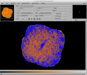 In order to filter the number of overlaid vectors down to a more useful number and size, various options in the GAIA: Polarimetry window can be used. First, select the Rendering tab on the left hand side. This will reveal a panel that will indicate which quantities are currently being used for the vector overlays. In this case, the Vector length is taken from the PI column of the table, and the Vector angles are taken from the ANG column (set the rotation to be 90 degrees for the vectors to represent the direction of the B-field ).
To filter out most of the extraneous vectors, click on the Selecting tab, and set the Expression field to be the following:
$I/$DI<10Press the “Enter” key after entering the above. The above expression simply selects the data points in the polarimetry table which have an associated non-polarized total intensity value (column I) less than 10 times that of its associated error value (column DI). All such catalogue entries will have changed color in the main Gaia plot window.
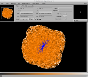
To remove the selected extraneous overlaid vectors, use the drop-down menu option Edit / Cut. This should leave just a small number of vectors clustering around the target object. In the central region of the map, it can already be seen that the level of vector ordering (and hence polarization) is quite low:
Note that it is possible to use more sophisticated entries for the Expression field, also including use of the “&” sign to include multiple filtering criteria.
To go back to the initial vector overlay in order to subsequently revise the filter criteria, simply use the drop-down menu option Edit / Undo three times. Feel free to experiment with the polarization overlay filtering. Note that it is also perfectly possible to specify criteria on the basis of other table columns, if desired. Be aware, however, that the errors given for the polarization components, DP and DQ, are dependent on the angular resolution and scale of the mapping, and should therefore be interpreted with care.
Another potentially useful option allows the user to change the length of the plotted vectors so that they do not overlap so much (via the Vector scale entry on the Rendering tab). Gaia can also be used to bin vector catalogues (see the Binning tab). Some users often bin their data up from the default 4″ pixel size to 12″, which is close to the JCMT beam size. This has the benefits of both reducing the noise level and reducing the number of vectors plotted, making the map clearer. As with any analysis technique, however, the user should be aware of the possibility that neighboring vectors might cancel out if the angle of polarization is changing rapidly in the region.
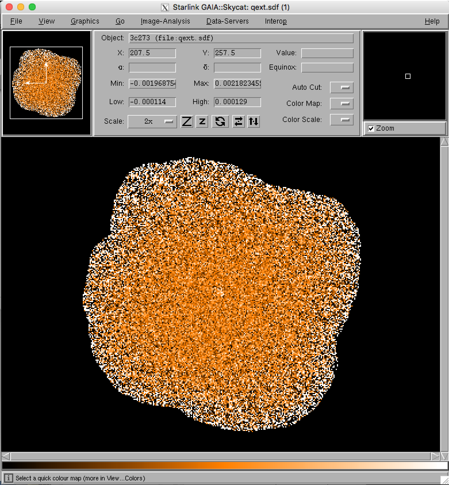
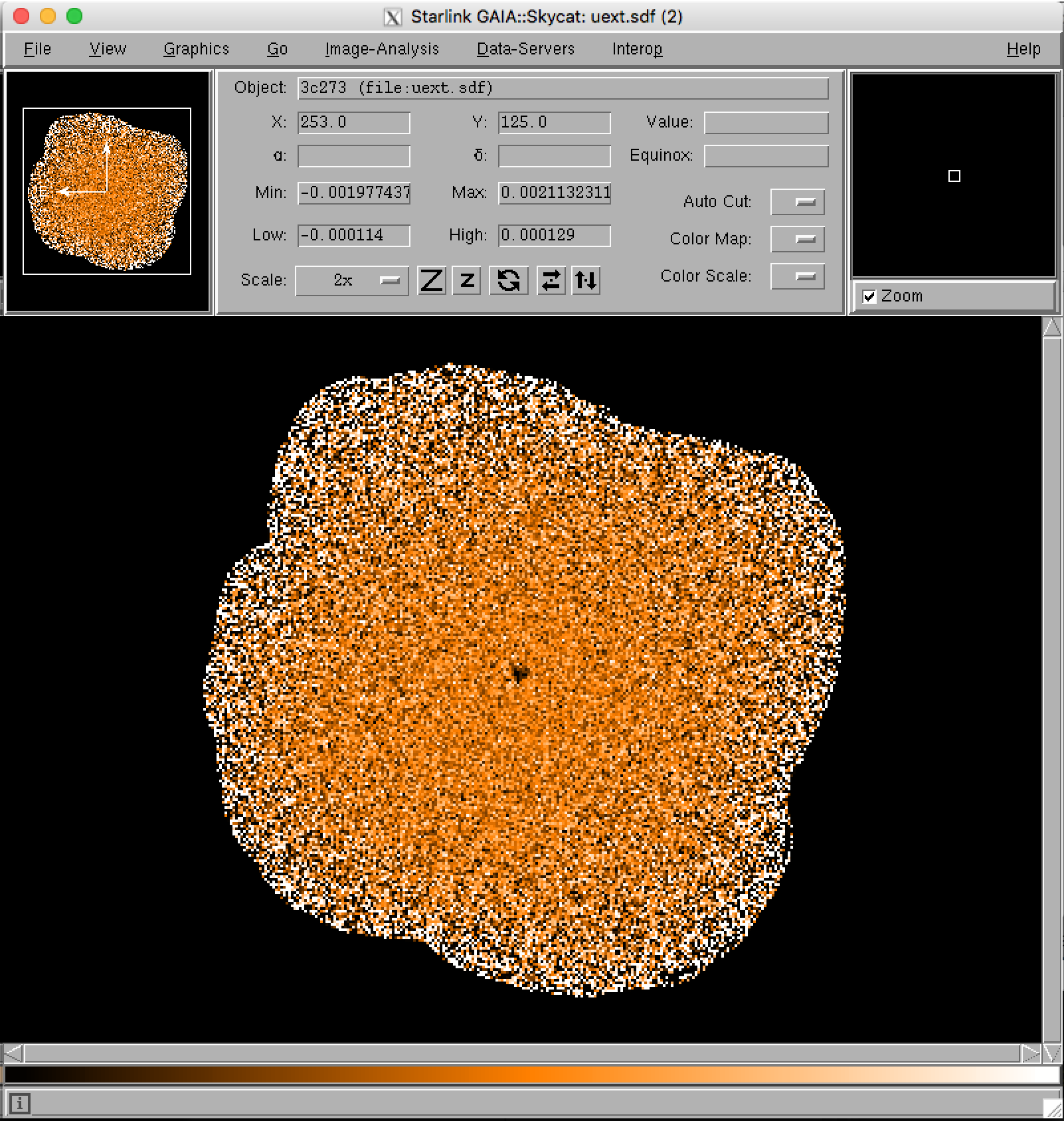
Furthermore, it should be noted that the above mapping example has been chosen primarily to simply illustrate what is possible. It is worth remembering that for most observations, the degree of polarization detected is small relative to the total intensity. This can be demonstrated with the example data by simply viewing the polarization images in Gaia. First, click on the Close button towards the lower right of the GAIA: Polarimetry window. In the main Gaia window, select the drop-down menu option File / Open and select the Q map file, qext.sdf, or the U map file, uext.sdf:
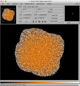
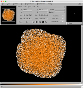
The central source appears comparatively faint in the resultant image due to the relatively low degree of source polarization.
POL-2 users intending to produce hardcopies or PDF/Postscript polarimetric vector map figures for publication purposes may also wish to experiment with using the Starlink POLPACK package. The POLPACK documentation (including usage examples) is available here.
- OPTIONAL ADDITIONAL MATERIAL: The pol2map command also has a number of other parameters that may also be used. More details of these can be obtained by typing:
smurfhelp pol2mapA small sample of other useful pol2map parameters are discussed here.
FCF: Due to the fact that the use of POL-2 reduces the throughput to SCUBA-2, additional compensations must be applied when calibrating POL-2 observational data. To convert POL-2 data to astronomical units such as mJy/beam a Flux Conversion Factor, FCF, must be applied to the data. For POL-2, the FCFs are quoted in terms of the SCUBA-2 FCFs (see here for more information on SCUBA-2 FCFs). The FCFs for POL-2 are found to be a factor of 1.35 and 1.96 times higher than the standard SCUBA-2 FCFs for 850 μm and 450 μm respectively. Unless explicitly specified otherwise using the optional FCF parameter, pol2map will use default values of 725.0 Jy/beam/pw and 962.0 Jy/beam/pw for 850 μm and 450 μm respectively.
PIXSIZE: The size of the pixels in the final maps can be changed by using the pol2map parameter pixsize. In practice, the pixel size to be used will probably be a trade-off between the ideal science goals of a given project and the practical amount of time needed for the observations (and reductions). In practice, recent projects have found a binned pixel size of 12″ to be appropriate. However, it may be worth noting that the difference between using 12″ pixels versus using the default 4″ pixel size and then binning the results on a 3×3 basis to produce a 12″ vector catalogue have not yet been deeply investigated at the time of writing. The use of 12″ pixels within makemap (inside pol2map) rather than 4″ pixels may have implications for the way in which makemap does or does not converge. We recommend using 4″ pixels and binning to 12″.
MAPVAR: changing the MAPVAR – changing between TRUE and FALSE is used to assist with noise estimation. MAPVAR=TURE will only provide useful numbers if multiple observations are provided in a reduction. MAPVAR=TRUE will look at variation in signal across different maps to estimate the noise. MAPVAR=TRUE uses bolometer variation to estimate the noise. MAPVAR=TRUE produced larger uncertainties (typically by factor 1.5-2). Currently recommended: MAPVAR=TRUE.
CONFIG, ICONFIG, QUCONFIG: More drastic modifications may be made to the various parts of the pol2map reduction workflow by (e.g.) tailoring the pol2map map-making processes. This can be done with the use of the config, iconfig and quconfig parameters. See the above help options for more details on how this is done.
The results of any such re-reductions can (of course) also be inspected with Gaia in the same manner as described above.
- ADDING NEW DATA TO PREVIOUSLY-REDUCED DATASETS: Although it is beyond the scope of this introductory tutorial, pol2map can be used process multiple observations, with the results automatically being combined into a single mosaic. It is also possible add in new observations to preexisting reductions of prior observations, avoiding the need to re-reduce the older observations. Please see Section 6.1 of the POL-2 Data Reduction Cookbook (Starlink document SC/22) for instructions on how to do this.
Other JCMT data reduction/analysis tutorials are available here.