


The following is a discussion of the factors that can attribute to variations between obtained rms values and predicted SCUBA-2 rms estimates:
Contents
Air Mass and ITC formula used
When we estimate the time required to spend on source we try to take into account the air mass at which the object is likely to be observed. Ideally you would always like to observe a source at zenith and at a night high elevation. The ITC’s equation as reported on the Calculating Integration Times page calculates an expected air mass which is slightly higher than that obtained by an object transiting at a given declination. This is also the case for the ITC Gui.
In the case of SCUBA-2 the estimation of an air-mass is further complicated because we avoid taking data with SCUBA-2 above an elevation of 70-75 degrees. This issue affects sources that have a Declination between +5 and +35 degrees. At these elevations the air mass is predicted (form the ITC formula) to be 1.15 or less, but this is clearly not the case.
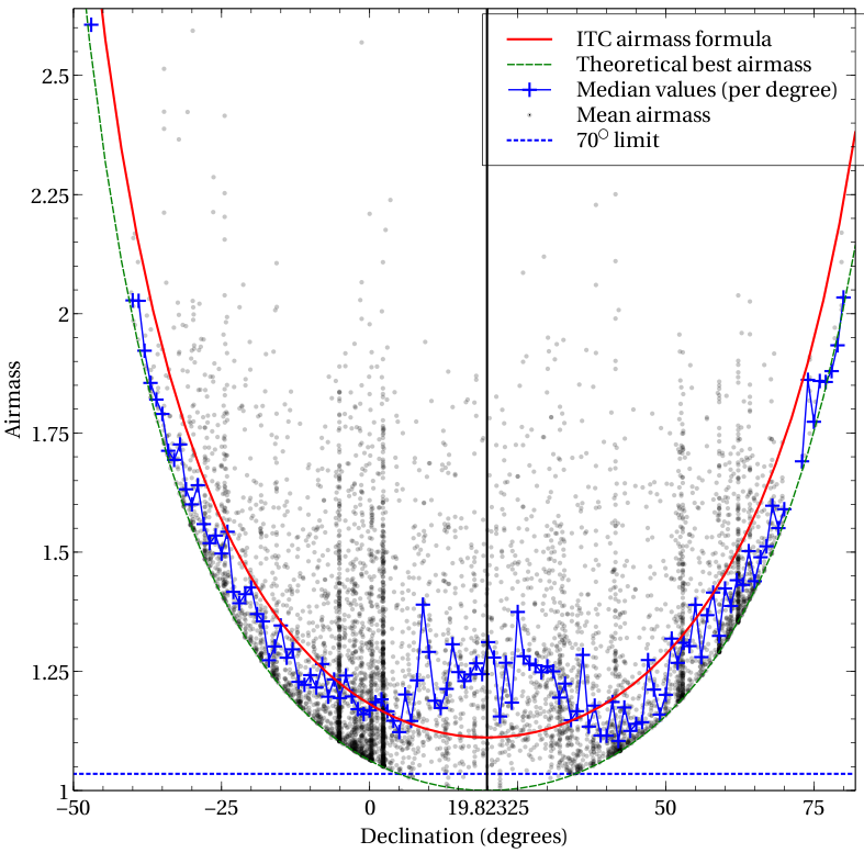
Figure displaying average air mass from a year’s worth of observations. We see that the air mass typically used in ITC estimations can underestimate the true air mass by up to 15%.
It is possible to determine the air mass at the start and end of an observation using:
>> fitsval file.sdf AMSTART
>> fitsval file.sdf AMEND
To see a record of the air mass throughout the observation it is possible to use the jcmtstate2cat command as outlined below.
Cropping
If you are comparing the rms obtained via the use of a tool such as PICARD’s SCUBA2_MAPSTATS then it may be important to consider the region used for estimating the noise in the map. In the following Daisy example we see that the region of highest exposure does not match perfectly with the centre of the map (the position the map is cropped for the noise estimation). This is particularly evident in the following image of a calibrator observation (these are short observations), and will emphasize any oddities such as the non-uniform distribution of bolometers that should get smoothed out over a longer integration.

rms from a Daisy observation (central 3′)
Exposure time from the same Daisy observation. Clearly see is that the map does not sit entirely in the centre of the cropped region.
Tau estimates
During JCMT observing the Water Vapor Monitor (WVM) inside the JCMT receiver cabin monitors the sky opacity for the same patch of sky that is observed. These measurements are key in helping to remove the atmospheric sky background from SCUBA-2 observations. For the most part the WVM is extremely reliable (see the plots below). We get a feeling for it’s reliability from comparison with the CSO’s WVM. The latter, however, stares at a fixed point in the atmosphere and does not have the time resolution of the WVM installed at the JCMT.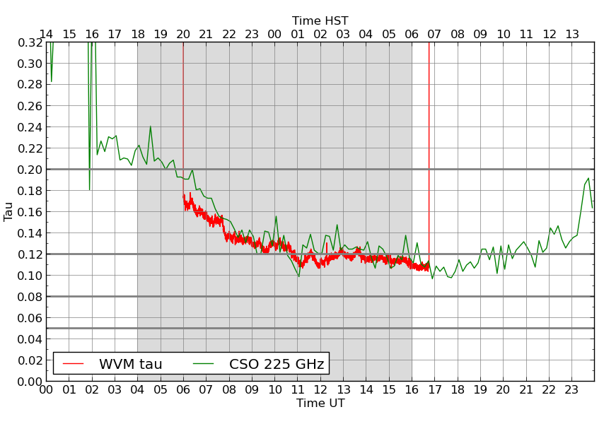
Unfortunately sometimes the JCMT’s WVM has issues and produces noisy spikes. When these occur (as shown below) it is necessary to base any SCUBA-2 extinction model from the CSO WVM. In the plot below the JCMT’s WVM is show in red, CSO in green and a fit to the CSO data is shown in blue. CSO WVM fits are produced for every night we observe with SCUBA-2 but generated fits are only used for a night when either the WVM was unavailable i.e. for maintenance or unusable due to noise spikes (such as the example below).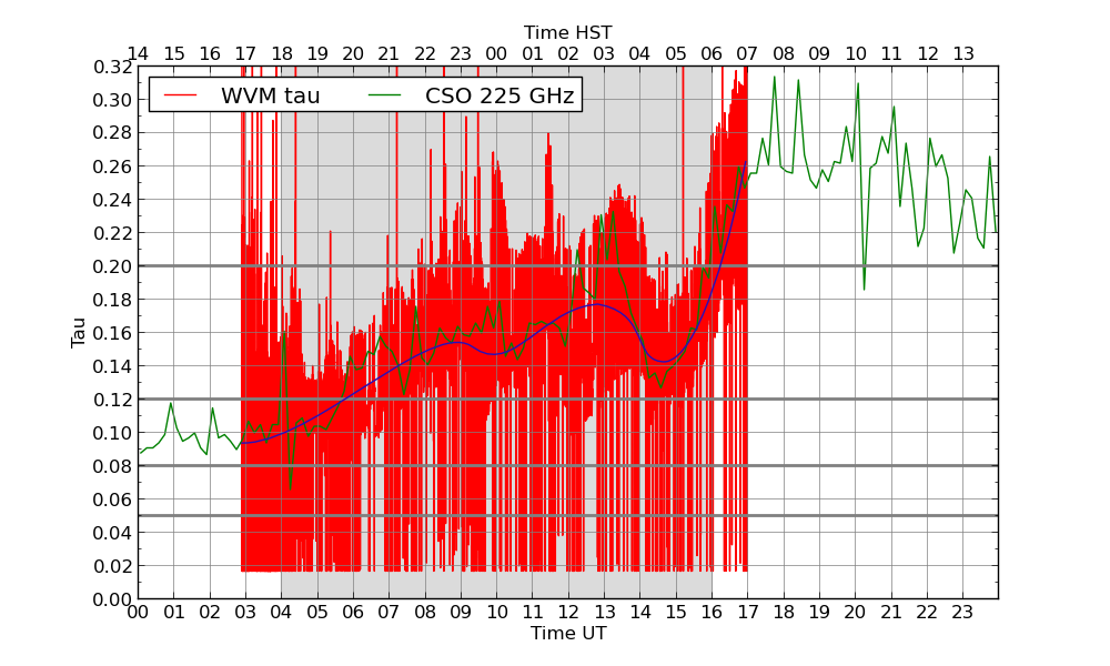 The map making software used to reduce data has access to dates when the WVM was having issues/offline. In these cases it uses the nightly CSO fits. To specifically control which model is used during reduction it is possible to use the ext.tausrc config parameter. The default value for ext.tausrc = auto. Allowed values are “auto”, “wvmraw”, “csotau” and “filtertau”.
Elevation issues
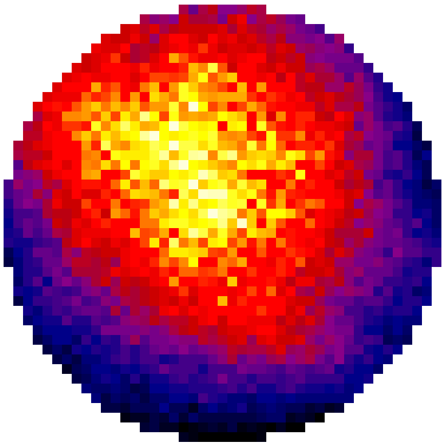
As is outlined in a sub section of the observing modes web page an elevation constraint 70 degrees is applied to observations. At high elevations the telescope struggles to make the tight turns at high speed required by the observing patterns. If you observation happened to be observed at a high elevation-close to this limit then it is possible that your exposure time and also noise coverage may be affected. This affect is clearly seen in the data if the usually circular pattern appears to be elongated. This problem appears confined to data taken in 2011 (when the exact observing mode method was being investigated).
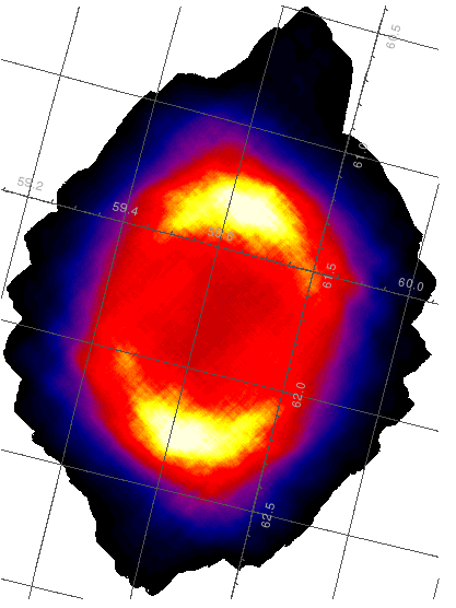
The exposure time map of a closed dome test observation taken at high elevation. This is an extreme example of an elevation issue.
NEPs
NEPs help serve as a measure of the arrays’ performance over the course of a night. The NEPs for each night we have SCUBA-2 data are plotted on the project page in the OMP. They are measured approximately every 30 seconds and plotted per sub-array. The image below shows a good night: the NEPs vary a bit throughout the night (which is natural), but do so in a way that is mostly smooth (except for the s8c array for observation 18) with almost no jumps in performance between observations.
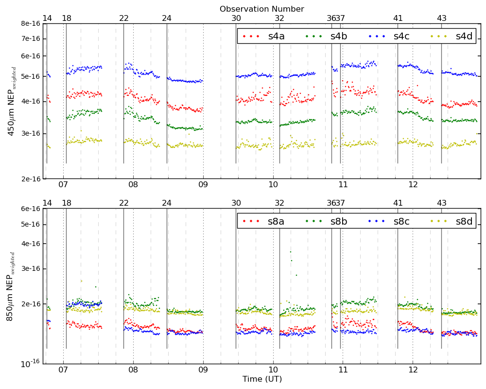
An example of a night where the NEP’s were well behaved.
The next image shows a worse night. Here the NEPs are jumping around quite a bit more, looking more like a swarm of points than a smooth-varying curve over time. There are some strange spikes on the scale of a few minutes in the last few observations (observation 63 and 68) as well.
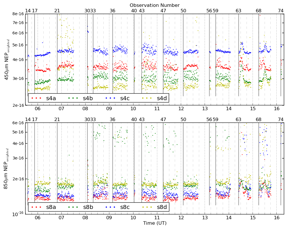
An example of a night where the NEPs were not good
Offline these variations can be investigated using ORAC-DR command: ASSESS_DATA_NOISE. Tweaks to the configuration file can eliminate or down weight noisy bolometers/sub-arrays with a trade off in noise.
Temperature Spikes
In very rare cases unexpected events occur at the JCMT which can feed into the noise component of an observation and it is good to be aware of these. Back in April 2012 we noticed some issues that were related to events where the FPU temperature increases and then exponentially returns to its steady state again. The origin of these particular temperature spikes was a caused by slip in the telescope elevation drive. Please note that temperature events form elevation slips were eliminated on 20120417.
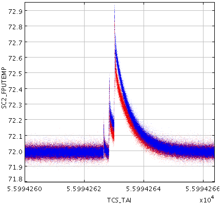
Focal Plane Unit temperatures (SC2_FPUTEMP) as measured at 450 and 850 microns. Normally constant we see a temperature excursion of over 0.5 mK.
Reduction method
When running the SCUBA-2 reduction software you can provide a number of different reduction recipes to use. Differences in rms based on the particular reduction methd (summit pipeline, vs off the shelf recipe, vs a bespoke reduction) can account for anywhere up to 10% or higher in some cases. This may be due to filters used, error estimates to remove small scale variations from the common mode, number of iterations etc. You may even find that a ‘good’ reduction in terms of visual appearance/science quality/lack of artifacts, might have a higher rms if more data is thrown away.
Diagnostic Tools
If you are worried about the quality of your data it is advisable to use some of the tools outlined below:
Quality statistics from the mapmaker
A first check might be to see how many samples made it into the final map. This can be done by inspecting the quality statistics displayed on the screen at the end of the final iteration, as shown:
smf_iteratemap: Iteration 7 / 40 ---------------
smf_iteratemap: Calculate time-stream model components
smf_iteratemap: Rebin residual to estimate MAP
smf_iteratemap: Calculate ast
--- Quality flagging statistics --------------------------------------------
 BADDA:   11322624 (37.56%),        1923 bolos  ,change          0 (+0.00%)
BADBOL:   11652352 (38.65%),        1979 bolos  ,change          0 (+0.00%)
 SPIKE:         30 ( 0.00%),                    ,change          0 (+0.00%)
DCJUMP:      13558 ( 0.04%),                    ,change          0 (+0.00%)
  STAT:     368640 ( 1.22%),          72 tslices,change          0 (+0.00%)
   COM:     295618 ( 0.98%),                    ,change          0 (+0.00%)
 NOISE:     111872 ( 0.37%),          19 bolos  ,change          0 (+0.00%)
Total samples available for map:   18178445, 60.30% of max (3087.37 bolos)
     Change from last report:          0, +0.00% of previous
smf_iteratemap: *** CHISQUARED = 0.973485660180563
smf_iteratemap: *** change: -4.25552926119899e-07
smf_iteratemap: *** NORMALIZED MAP CHANGE: 0.0323018 (mean) 0.0519139 (max)
smf_iteratemap: ****** Completed in 7 iterations
smf_iteratemap: ****** Solution CONVERGED
For more information regarding the map maker and for diagnostic tools for advanced users please see the SCUBA-2 data reduction book.
Telescope status
To check the status of an observation in detail can be done by running the command: jcmtstate2cat on the raw data:
>> jcmtstate2cat /directory/raw/data/files.sdf > state.tst
>> topcat -f tst state.tst
and plotting one parameter against another i.e.
- RA vs Dec
- to look at mapping pattern on source
- Az vs El
- to look at mapping pattern on sky
- Id vs WVMTAU
- to look for WVM problems
- Id vs SC2_FPUTEMP
- to look at focal plane temperature
- Id vs TCS_AIRMASS
- to look at the change in air mass during an observation
Config file
To display the name and value of one or all configuration parameters either from a configuration file or from the history of an NDF file use the KAPPA command configecho. See here for more information on map provenance & configuration parameters.
The first example below will return the value of numiter from the map 850map.sdf. The second example will display the values of all the parameters in 850map.sdf and will prefix them with a ‘+’ if they differ from the the values given in dimmconfig.lis.
>> configecho name=numiter config=! ndf=file.sdf
>> configecho name=! config=^dimmconfig.lis ndf=file.sdf
If you wish to compare differences between maps (i.e. maps with large differences in rms’s) you can simply use the configmeld command:
>> configmeld file1.sdf files2.sdf
>> configmeld file1.sdf ^dimmconfig2.lis
Sometimes it is useful to write out each iteration of the map maker to see how the map maker progresses during a reduction. For more information on writing out models and intermediate maps click here.
Checking array noise
To check how the noise changes on an array over an observation it is possible to use the ORAC-DR command: ASSESS_DATA_NOISE. As an example the following asses the noise on the 450um data for observation 68 taken on the 20130329.
>> oracdr_scuba2_450 -cwd  20130329
>> oracdr -log sf -recpars params.ini -loop flag -list 68 ASSESS_DATA_NOISE
with params.ini containing:
[ASSESS_DATA_NOISE]
NOISE_CALC = each
NOISE_CFG = dimmconfig.lis
Where NOISE_CFG is the config file used on the data, NOISE_CALC = each, will calculate the noise on each science observation. The outputs from the above are:
>> log.scinoise450
>> log.bolonoise
>> log.nep
which can be viewed using TOPCAT.